H.264 and MPEG-4 Video Compression phần 3 pps
Bạn đang xem bản rút gọn của tài liệu. Xem và tải ngay bản đầy đủ của tài liệu tại đây (632.04 KB, 31 trang )
VIDEO CODING CONCEPTS
•
38
2
4 6 8
10
12 14
16
2
4
6
8
10
12
14
16
Figure 3.16 Close-up of reference region
5 10 15 20 25 30
5
10
15
20
25
30
Figure 3.17 Reference region interpolated to half-pixel positions
TEMPORAL MODEL
•
39
Integer search positions
Best integer match
Half-pel search positions
Best half-pel match
Quarter-pel search positions
Best quarter-pel match
Key :
Figure 3.18 Integer, half-pixel and quarter-pixel motion estimation
Figure 3.19 Residual (4 × 4 blocks, half-pixel compensation)
Figure 3.20 Residual (4 × 4 blocks, quarter-pixel compensation)
VIDEO CODING CONCEPTS
•
40
Table 3.1 SAE of residual frame after motion compensation (16 × 16 block size)
Sequence No motion compensation Integer-pel Half-pel Quarter-pel
‘Violin’, QCIF 171945 153475 128320 113744
‘Grasses’, QCIF 248316 245784 228952 215585
‘Carphone’, QCIF 102418 73952 56492 47780
Figure 3.21 Motion vector map (16 × 16 blocks, integer vectors)
Some examples of the performance achieved by sub-pixel motion estimation and com-
pensation are given in Table 3.1. A motion-compensated reference frame (the previous frame
in the sequence) is subtracted from the current frame and the energy of the residual (approx-
imated by the Sum of Absolute Errors, SAE) is listed in the table. A lower SAE indicates
better motion compensation performance. In each case, sub-pixel motion compensation gives
improved performance compared with integer-sample compensation. The improvement from
integer to half-sample is more significant than the further improvement from half- to quarter-
sample. The sequence ‘Grasses’ has highly complex motion and is particularly difficult to
motion-compensate, hence the large SAE; ‘Violin’ and ‘Carphone’ are less complex and
motion compensation produces smaller SAE values.
TEMPORAL MODEL
•
41
Figure 3.22 Motion vector map (4 × 4 blocks, quarter-pixel vectors)
Searching for matching 4 × 4 blocks with quarter-sample interpolation is considerably
more complex than searching for 16 × 16 blocks with no interpolation. In addition to the extra
complexity, there is a coding penalty since the vector for every block must be encoded and
transmitted to the receiver in order to reconstruct the image correctly. As the block size is
reduced, the number of vectors that have to be transmitted increases. More bits are required to
represent half- or quarter-sample vectors because thefractionalpart of the vector (e.g. 0.25, 0.5)
must be encoded as well as the integer part. Figure 3.21 plots the integer motion vectors that are
required to be transmitted along with the residual of Figure 3.13. The motion vectors required
for the residual of Figure 3.20 (4 × 4 block size) are plotted in Figure 3.22, in which there are 16
times as many vectors, each represented by two fractional numbers DX and DY with quarter-
pixel accuracy. There is therefore a tradeoff in compression efficiency associated with more
complex motion compensation schemes, since more accurate motion compensation requires
more bits to encode the vector field but fewer bits to encode the residual whereas less accurate
motion compensation requires fewer bits for the vector field but more bits for the residual.
3.3.7 Region-based Motion Compensation
Moving objects in a ‘natural’ video scene are rarely aligned neatly along block boundaries
but are likely to be irregular shaped, to be located at arbitrary positions and (in some cases)
to change shape between frames. This problem is illustrated by Figure 3.23, in which the
VIDEO CODING CONCEPTS
•
42
Problematic
macroblock
Reference frame
Current frame
Possible
matching
positions
Figure 3.23 Motion compensation of arbitrary-shaped moving objects
oval-shaped object is moving and the rectangular object is static. It is difficult to find a good
match in the reference frame for the highlighted macroblock, because it covers part of the
moving object and part of the static object. Neither of the two matching positions shown in
the reference frame are ideal.
It may be possible to achieve better performance by motion compensating arbitrary
regions of the picture (region-based motion compensation). For example, if we only attempt
to motion-compensate pixel positions inside the oval object then we can find a good match
in the reference frame. There are however a number of practical difficulties that need to be
overcome in order to use region-based motion compensation, including identifying the region
boundaries accurately and consistently, (segmentation) signalling (encoding) the contour of
the boundary to the decoder and encoding the residual after motion compensation. MPEG-4
Visual includes a number of tools that support region-based compensation and coding and
these are described in Chapter 5.
3.4 IMAGE MODEL
A natural video image consists of a grid of sample values. Natural images are often difficult to
compress in their original form because of the high correlation between neighbouring image
samples. Figure 3.24 shows the two-dimensional autocorrelation function of a natural video
image (Figure 3.4) in which the height of the graph at each position indicates the similarity
between the original image and a spatially-shifted copy of itself. The peak at the centre of the
figure corresponds to zero shift. As the spatially-shifted copy is moved away from the original
image in any direction, the function drops off as shown in the figure, with the gradual slope
indicating that image samples within a local neighbourhood are highly correlated.
A motion-compensated residual image such as Figure3.20 has an autocorrelation function
(Figure 3.25) that drops off rapidly as the spatial shift increases, indicating that neighbouring
samples are weakly correlated. Efficient motion compensation reduces local correlation in the
residual making it easier to compress than the original video frame. The function of the image
IMAGE MODEL
•
43
8
6
4
2
100
50
0
0
50
X 10
8
10
0
Figure 3.24 2D autocorrelation function of image
X 10
5
6
4
2
0
−2
20
10
00
10
20
Figure 3.25 2D autocorrelation function of residual
VIDEO CODING CONCEPTS
•
44
Raster
scan
order
Current pixel
B C
A X
Figure 3.26 Spatial prediction (DPCM)
model is to decorrelate image or residual data further and to convert it into a form that can be
efficiently compressed using an entropy coder. Practical image models typically have three
main components, transformation (decorrelates and compacts the data), quantisation (reduces
the precision of the transformed data) and reordering (arranges the data to group together
significant values).
3.4.1 Predictive Image Coding
Motion compensation is an example of predictive coding in which an encoder creates a pre-
diction of a region of the current frame based on a previous (or future) frame and subtracts
this prediction from the current region to form a residual. If the prediction is successful, the
energy in the residual is lower than in the original frame and the residual can be represented
with fewer bits.
In a similar way, a prediction of an image sample or region may be formed from
previously-transmitted samples in the same image or frame. Predictive coding was used as
the basis for early image compression algorithms and is an important component of H.264
Intra coding (applied in the transform domain, see Chapter 6). Spatial prediction is sometimes
described as ‘Differential Pulse Code Modulation’ (DPCM), a term borrowed from a method
of differentially encoding PCM samples in telecommunication systems.
Figure 3.26 shows a pixel X that is to be encoded. If the frame is processed in raster order,
then pixels A, B and C (neighbouring pixels in the current and previous rows) are available in
both the encoder and the decoder (since these should already have been decoded before X).
The encoder forms a prediction for X based on some combination of previously-coded pixels,
subtracts this prediction from X and encodes the residual (the result of the subtraction). The
decoder forms the same prediction and adds the decoded residual to reconstruct the pixel.
Example
Encoder prediction P(X) = (2A + B + C)/4
Residual R(X) = X – P(X) is encoded and transmitted.
Decoder decodes R(X) and forms the same prediction: P(X) = (2A + B + C)/4
Reconstructed pixel X = R(X) + P(X)
IMAGE MODEL
•
45
If the encoding process is lossy (e.g. if the residual is quantised – see section 3.4.3) then the
decoded pixels A
,B
and C
may not be identical to the original A, B and C (due to losses
during encoding) and so the above process could lead to a cumulative mismatch (or ‘drift’)
between the encoder and decoder. In this case, the encoder should itself decode the residual
R
(X) and reconstruct each pixel.
The encoder uses decoded pixels A
,B
and C
to form the prediction, i.e. P(X) = (2A
+
B
+ C
)/4 in the above example. In this way, both encoder and decoder use the same prediction
P(X) and drift is avoided.
The compression efficiency of this approach depends on the accuracy of the prediction
P(X). If the prediction is accurate (P(X) is a close approximation of X) then the residual energy
will be small. However, it is usually not possible to choose a predictor that works well for all
areas of a complex image and better performance may be obtained by adapting the predictor
depending on the local statistics of the image (for example, using different predictors for areas
of flat texture, strong vertical texture, strong horizontal texture, etc.). It is necessary for the
encoder to indicate the choice of predictor to the decoder and so there is a tradeoff between
efficient prediction and the extra bits required to signal the choice of predictor.
3.4.2 Transform Coding
3.4.2.1 Overview
The purpose of the transform stage in an image or video CODEC is to convert image or
motion-compensated residual data into another domain (the transform domain). The choice
of transform depends on a number of criteria:
1. Data in the transform domain should be decorrelated (separated into components with
minimal inter-dependence) and compact (most of the energy in the transformed data should
be concentrated into a small number of values).
2. The transform should be reversible.
3. The transform should be computationally tractable (low memory requirement, achievable
using limited-precision arithmetic, low number of arithmetic operations, etc.).
Many transforms have been proposed for image and video compression and the most pop-
ular transforms tend to fall into two categories: block-based and image-based. Examples
of block-based transforms include the Karhunen–Loeve Transform (KLT), Singular Value
Decomposition (SVD) and the ever-popular Discrete Cosine Transform (DCT) [3]. Each of
these operate on blocks of N × N image or residual samples and hence the image is processed
in units of a block. Block transforms have low memory requirements and are well-suited to
compression of block-based motion compensation residuals but tend to suffer from artefacts
at block edges (‘blockiness’). Image-based transforms operate on an entire image or frame
(or a large section of the image known as a ‘tile’). The most popular image transform is
the Discrete Wavelet Transform (DWT or just ‘wavelet’). Image transforms such as the DWT
have been shown to out-perform block transforms for still image compression but they tend to
have higher memory requirements (because the whole image or tile is processed as a unit) and
VIDEO CODING CONCEPTS
•
46
do not ‘fit’ well with block-based motion compensation. The DCT and the DWT both feature
in MPEG-4 Visual (and a variant of the DCT is incorporated in H.264) and are discussed
further in the following sections.
3.4.2.2 DCT
The Discrete Cosine Transform (DCT) operates on X, a block of N × N samples (typi-
cally image samples or residual values after prediction) and creates Y,anN × N block
of coefficients. The action of the DCT (and its inverse, the IDCT) can be described in
terms of a transform matrix A. The forward DCT (FDCT) of an N × N sample block is
given by:
Y = AXA
T
(3.1)
and the inverse DCT (IDCT) by:
X = A
T
YA (3.2)
where X is a matrix of samples, Y is a matrix of coefficients and A is an N × N transform
matrix. The elements of A are:
A
ij
= C
i
cos
(2 j + 1)iπ
2N
where C
i
=
1
N
(i = 0), C
i
=
2
N
(i > 0) (3.3)
Equation 3.1 and equation 3.2 may be written in summation form:
Y
xy
= C
x
C
y
N −1
i=0
N −1
j=0
X
ij
cos
(2 j + 1)yπ
2N
cos
(2i + 1)xπ
2N
(3.4)
X
ij
=
N −1
x=0
N −1
y=0
C
x
C
y
Y
xy
cos
(2 j + 1)yπ
2N
cos
(2i + 1)xπ
2N
(3.5)
Example: N = 4
The transform matrix A fora4× 4 DCT is:
A =
1
2
cos
(
0
)
1
2
cos
(
0
)
1
2
cos
(
0
)
1
2
cos
(
0
)
1
2
cos
π
8
1
2
cos
3π
8
1
2
cos
5π
8
1
2
cos
7π
8
1
2
cos
2π
8
1
2
cos
6π
8
1
2
cos
10π
8
1
2
cos
14π
8
1
2
cos
3π
8
1
2
cos
9π
8
1
2
cos
15π
8
1
2
cos
21π
8
(3.6)
IMAGE MODEL
•
47
The cosinefunction is symmetrical and repeats after 2π radians and hence A can be simplified
to:
A =
1
2
1
2
1
2
1
2
1
2
cos
π
8
1
2
cos
3π
8
−
1
2
cos
3π
8
−
1
2
cos
π
8
1
2
−
1
2
−
1
2
1
2
1
2
cos
3π
8
−
1
2
cos
π
8
1
2
cos
π
8
−
1
2
cos
3π
8
(3.7)
or
A =
aaaa
bc−c −b
a −a −aa
c −bbc
where
a =
1
2
b =
1
2
cos
π
8
c =
1
2
cos
3π
8
(3.8)
Evaluating the cosines gives:
A =
0.50.50.50.5
0.653 0.271 0.271 −0.653
0.5 −0.5 −0.50.5
0.271 −0.653 −0.653 0.271
The output of a two-dimensional FDCT is a set of N × N coefficients representing the image
block data in the DCT domain and these coefficients can be considered as ‘weights’ of a set
of standard basis patterns. The basis patterns for the 4 × 4 and 8 × 8 DCTs are shown in
Figure 3.27 and Figure 3.28 respectively and are composed of combinations of horizontal and
vertical cosine functions. Any image block may be reconstructed by combining all N × N
basis patterns, with each basis multiplied by the appropriate weighting factor (coefficient).
Example 1 Calculating the DCT of a 4 × 4 block
X is 4 × 4 block of samples from an image:
j = 0123
i = 0 5 11 8 10
1 9 8412
2 1 10 11 4
3 19 6 15 7
VIDEO CODING CONCEPTS
•
48
Figure 3.27 4 × 4 DCT basis patterns
Figure 3.28 8 × 8 DCT basis patterns
IMAGE MODEL
•
49
The Forward DCT of X is given by: Y = AXA
T
. The first matrix multiplication, Y
= AX, cor-
responds to calculating the one-dimensional DCT of each column of X. For example, Y
00
is
calculated as follows:
Y
00
= A
00
X
00
+ A
01
X
10
+ A
02
X
20
+ A
03
X
30
= (0.5 ∗ 5) + (0.5 ∗ 9) + (0.5 ∗ 1)
+ (0.5 ∗ 19) = 17.0
The complete result of the column calculations is:
Y
= AX =
17 17.51916.5
−6.981 2.725 −6.467 4.125
7 −0.540.5
−9.015 2.660 2.679 −4.414
Carrying out the second matrix multiplication, Y = Y
A
T
, is equivalent to carrying out a 1-D DCT
on each row of Y
:
Y = AXA
T
=
35.0 −0.079 −1.51.115
−3.299 −4.768 0.443 −9.010
5.53.029 2.04.699
−4.045 −3.010 −9.384 −1.232
(Note: the order of the row and column calculations does not affect the final result).
Example 2 Image block and DCT coefficients
Figure 3.29 shows an image with a 4 × 4 block selected and Figure 3.30 shows the block in
close-up, together with the DCT coefficients. The advantage of representing the block in the DCT
domain is not immediately obvious since there is no reduction in the amount of data; instead of
16 pixel values, we need to store 16 DCT coefficients. The usefulness of the DCT becomes clear
when the block is reconstructed from a subset of the coefficients.
Figure 3.29 Image section showing 4 × 4 block
VIDEO CODING CONCEPTS
•
50
75
80
98
126
114
137
151
159
88
176
181
178
68
156
181
181
537.2537.2
-106.1
-42.7
-20.2
-76.0
35.0
46.5
12.9
-12.7
10.3
3.9
-7.8
-6.1
-9.8
-8.5
Original block
-54.8
DCT coefficients
Figure 3.30 Close-up of 4 × 4 block; DCT coefficients
Setting all the coefficients to zero except the most significant (coefficient 0,0, described as
the ‘DC’ coefficient) and performing the IDCT gives the output block shown in Figure 3.31(a), the
mean of the original pixel values. Calculating the IDCT of the two most significant coefficients
gives the block shown in Figure 3.31(b). Adding more coefficients before calculating the IDCT
produces a progressively more accurate reconstruction of the original block and by the time five
coefficients are included (Figure 3.31(d)), the reconstructed block is a reasonably close match to
the original. Hence it is possible to reconstruct an approximate copy of the block from a subset of
the 16 DCT coefficients. Removing the coefficients with insignificant magnitudes (for example
by quantisation, see Section 3.4.3) enables image data to be represented with a reduced number
of coefficient values at the expense of some loss of quality.
3.4.2.3 Wavelet
The popular ‘wavelet transform’ (widely used in image compression is based on sets of filters
with coefficients that are equivalent to discrete wavelet functions [4]. The basic operation of a
discrete wavelet transform is as follows, applied to a discrete signal containing N samples. A
pair of filters are applied to the signal to decompose it into a low frequency band (L) and a high
frequency band (H). Each band is subsampled by a factor of two, so that the two frequency
bands each contain N/2 samples. With the correct choice of filters, this operation is reversible.
This approach may be extended to apply to a two-dimensional signal such as an intensity
image (Figure 3.32). Each row of a 2D image is filtered with a low-pass and a high-pass
filter (L
x
and H
x
) and the output of each filter is down-sampled by a factor of two to produce
the intermediate images L and H. L is the original image low-pass filtered and downsampled
in the x-direction and H is the original image high-pass filtered and downsampled in the x-
direction. Next, each column of these new images is filtered with low- and high-pass filters
(L
y
and H
y
) and down-sampled by a factor of two to produce four sub-images (LL, LH, HL
and HH). These four ‘sub-band’ images can be combined to create an output image with the
same number of samples as the original (Figure 3.33). ‘LL’ is the original image, low-pass
filtered in horizontal and vertical directions and subsampled by a factor of 2. ‘HL’ is high-pass
filtered in the vertical direction and contains residual vertical frequencies, ‘LH’ is high-pass
filtered in the horizontal direction and contains residual horizontal frequencies and ‘HH’ is
high-pass filtered in both horizontal and vertical directions. Between them, the four subband
IMAGE MODEL
•
51
134
134
134
134
134
134
134
134
134
134
134
134
134
134
134
134
100
120
149
169
100
120
149
169
100
120
149
169
100
120
149
169
75
95
124
144
89
110
138
159
110
130
159
179
124
145
173
194
1 coefficient
(a) (b)
(c) (d)
2 coefficients
5 coefficients
76
66
95
146
109
117
146
179
117
150
179
187
96
146
175
165
3 coefficients
Figure 3.31 Block reconstructed from (a) one, (b) two, (c) three, (d) five coefficients
images contain all of the information present in the original image but the sparse nature of the
LH, HL and HH subbands makes them amenable to compression.
In an image compression application, the two-dimensional wavelet decomposition de-
scribed above is applied again to the ‘LL’ image, forming four new subband images. The
resulting low-pass image (always the top-left subband image) is iteratively filtered to create
a tree of subband images. Figure 3.34 shows the result of two stages of this decomposi-
tion and Figure 3.35 shows the result of five stages of decomposition. Many of the samples
(coefficients) in the higher-frequency subband images are close to zero (near-black) and it is
possible to achieve compression by removing these insignificant coefficients prior to trans-
mission. At the decoder, the original image is reconstructed by repeated up-sampling, filtering
and addition (reversing the order of operations shown in Figure 3.32).
3.4.3 Quantisation
A quantiser maps a signal with a range of values X to a quantised signal with a reduced range
of values Y. It should be possible to represent the quantised signal with fewer bits than the
original since the range of possible values is smaller. A scalar quantiser maps one sample of
the input signal to one quantised output value and a vector quantiser maps a group of input
samples (a ‘vector’) to a group of quantised values.
VIDEO CODING CONCEPTS
•
52
Lx
Hx
Ly
Hy
Ly
Hy
down-
sample
down-
sample
down-
sample
down-
sample
down-
sample
down-
sample
LL
LH
HL
HH
L
H
Figure 3.32 Two-dimensional wavelet decomposition process
LL
HL
LH
HH
Figure 3.33 Image after one level of decomposition
3.4.3.1 Scalar Quantisation
A simple example of scalar quantisation is the process of rounding a fractional number to the
nearest integer, i.e. the mapping is from R to Z . The process is lossy (not reversible) since it is
not possible to determine the exact value of the original fractional number from the rounded
integer.
IMAGE MODEL
•
53
Figure 3.34 Two-stage wavelet decomposition of image
Figure 3.35 Five-stage wavelet decomposition of image
A more general example of a uniform quantiser is:
FQ = round
X
QP
Y = FQ.QP
(3.9)
VIDEO CODING CONCEPTS
•
54
where QP is a quantisation ‘step size’. The quantised output levels are spaced at uniform
intervals of QP (as shown in the following example).
Example Y = QP.round(X/QP)
Y
X QP = 1 QP = 2 QP = 3 QP = 5
−4 −4 −4 −3 −5
−3 −3 −2 −3 −5
−2 −2 −2 −30
−1 −1000
00000
11000
22230
33235
44435
55465
66665
77665
888910
998910
10 10 10 9 10
11 11 10 12 10
······
Figure 3.36 shows two examples of scalar quantisers, a linear quantiser (with a linear
mapping between input and output values) and a nonlinear quantiser that has a ‘dead zone’
about zero (in which small-valued inputs are mapped to zero).
IMAGE MODEL
•
55
1
243
-1
-2
- 3
-4
1
2
3
4
-2
-1
-3
-4
Output
0
Input
1
2
3
4
-1
-2
-3
-4
1
2
3
4
-1
-2
-3
Output
0
dead
zone
-4
linear
nonlinear
Input
Figure 3.36 Scalar quantisers: linear; nonlinear with dead zone
In image and video compression CODECs, the quantisation operation is usually made up
of two parts: a forward quantiser FQ in the encoder and an ‘inverse quantiser’ or (IQ) in the de-
coder (in fact quantization is not reversible and so a more accurate term is ‘scaler’ or ‘rescaler’).
A critical parameter is the step size QP between successive re-scaled values. If the step size
is large, the range of quantised values is small and can therefore be efficiently represented
(highly compressed) during transmission, but the re-scaled values are a crude approximation
to the original signal. If the step size is small, the re-scaled values match the original signal
more closely but the larger range of quantised values reduces compression efficiency.
Quantisation may be used to reduce the precision of image data after applying a transform
such as the DCT or wavelet transform removing remove insignificant values such as near-zero
DCT or wavelet coefficients. The forward quantiser in an image or video encoder is designed
to map insignificant coefficient values to zero whilst retaining a reduced number of significant,
nonzero coefficients. The output of a forward quantiser is typically a ‘sparse’ array of quantised
coefficients, mainly containing zeros.
3.4.3.2 Vector Quantisation
A vector quantiser maps a set of input data (such as a block of image samples) to a single value
(codeword) and, at the decoder, each codeword maps to an approximation to the original set of
input data (a ‘vector’). The set of vectors are stored at the encoder and decoder in a codebook.
A typical application of vector quantisation to image compression [5] is as follows:
1. Partition the original image into regions (e.g. M × N pixel blocks).
2. Choose a vector from the codebook that matches the current region as closely as possible.
3. Transmit an index that identifies the chosen vector to the decoder.
4. At the decoder, reconstruct an approximate copy of the region using the selected vector.
A basic system is illustrated in Figure 3.37. Here, quantisation is applied in the spatial domain
(i.e. groups of image samples are quantised as vectors) but it could equally be applied to
VIDEO CODING CONCEPTS
•
56
Find best
match
Codebook
Vector 1
Vector 2
Vector N
Look up
Codebook
Vector 1
Vector 2
Vector N
Input
block
Output
block
Encoder Decoder
Transmit
code index
Figure 3.37 Vector quantisation
motion compensated and/or transformed data. Key issues in vector quantiser design include
the design of the codebook and efficient searching of the codebook to find the optimal
vector.
3.4.4 Reordering and Zero Encoding
Quantised transform coefficients are required to be encoded as compactly as possible prior
to storage and transmission. In a transform-based image or video encoder, the output of
the quantiser is a sparse array containing a few nonzero coefficients and a large number of
zero-valued coefficients. Reordering (to group together nonzero coefficients) and efficient
representation of zero coefficients are applied prior to entropy encoding. These processes are
described for the DCT and wavelet transform.
3.4.4.1 DCT
Coefficient Distribution
The significant DCT coefficients of a block of image or residual samples are typically the
‘low frequency’ positions around the DC (0,0) coefficient. Figure 3.38 plots the probability
of nonzero DCT coefficients at each position in an 8 × 8 block in a QCIF residual frame
(Figure 3.6). The nonzero DCT coefficients are clustered around the top-left (DC) coefficient
and the distribution is roughly symmetrical in the horizontal and vertical directions. For a
residual field (Figure 3.39), Figure 3.40 plots the probability of nonzero DCT coefficients;
here, the coefficients are clustered around the DC position but are ‘skewed’, i.e. more nonzero
IMAGE MODEL
•
57
1 2 3 4 5 6 7 8
1
2
3
4
5
6
7
8
Figure 3.38 8 × 8 DCT coefficient distribution (frame)
Figure 3.39 Residual field picture
coefficients occur along the left-hand edge of the plot. This is because the field picture has a
stronger high-frequency component in the vertical axis (due to the subsampling in the vertical
direction) resulting in larger DCT coefficients corresponding to vertical frequencies (refer to
Figure 3.27).
Scan
After quantisation, the DCT coefficients for a block are reordered to group together nonzero
coefficients, enabling efficient representation of the remaining zero-valued quantised coeffi-
cients. The optimum reordering path (scan order) depends on the distribution of nonzero DCT
coefficients. For a typical frame block with a distribution similar to Figure 3.38, a suitable
scan order is a zigzag starting from the DC (top-left) coefficient. Starting with the DC coef-
ficient, each quantised coefficient is copied into a one-dimensional array in the order shown
in Figure 3.41. Nonzero coefficients tend to be grouped together at the start of the reordered
array, followed by long sequences of zeros.
VIDEO CODING CONCEPTS
•
58
1 2 3 4 5 6 7 8
1
2
3
4
5
6
7
8
Figure 3.40 8 × 8 DCT coefficient distribution (field)
The zig-zag scan may not be ideal for a field block because of the skewed coefficient
distribution (Figure 3.40) and a modified scan order such as Figure 3.42 may be more effective,
in which coefficients on the left-hand side of the block are scanned before those on the right-
hand side.
Run-Level Encoding
The output of the reordering process is an array that typically contains one or more clusters
of nonzero coefficients near the start, followed by strings of zero coefficients. The large
number of zero values may be encoded to represent them more compactly, for example
by representing the array as a series of (run, level) pairs where run indicates the number
of zeros preceding a nonzero coefficient and level indicates the magnitude of the nonzero
coefficient.
Example
Input array: 16,0,0,−3,5,6,0,0,0,0,−7,
Output values: (0,16),(2,−3),(0,5),(0,6),(4,−7)
Each of these output values (a run-level pair) is encoded as a separate symbol by the entropy
encoder.
Higher-frequency DCT coefficients are very often quantised to zero and so a reordered
block will usually end in a run of zeros. A special case is required to indicate the final
nonzero coefficient in a block. In so-called ‘Two-dimensional’ run-level encoding is used,
each run-level pair is encoded as above and a separate code symbol, ‘last’, indicates the end of
the nonzero values. If ‘Three-dimensional’ run-level encoding is used, each symbol encodes
IMAGE MODEL
•
59
Figure 3.41 Zigzag scan order (frame block)
start
etc.
end
Figure 3.42 Zigzag scan order (field block)
three quantities, run, level and last. In the example above, if –7 is the final nonzero coefficient,
the 3D values are:
(0, 16, 0), (2, −3, 0), (0, 5, 0), (0, 6, 0), (4, −7, 1)
The 1 in the final code indicates that this is the last nonzero coefficient in the block.
3.4.4.2 Wavelet
Coefficient Distribution
Figure 3.35 shows a typical distribution of 2D wavelet coefficients. Many coefficients in
higher sub-bands (towards the bottom-right of the figure) are near zero and may be quantised
VIDEO CODING CONCEPTS
•
60
Layer 1 Layer 2
Figure 3.43 Wavelet coefficient and ‘children’
to zero without significant loss of image quality. Nonzero coefficients tend to correspond to
structures in the image; for example, the violin bow appears as a clear horizontal structure in
all the horizontal and diagonal subbands. When a coefficient in a lower-frequency subband is
nonzero, there is a strong probability that coefficients in the corresponding position in higher-
frequency subbands will also be nonzero. We may consider a ‘tree’ of nonzero quantised
coefficients, starting with a ‘root’ in a low-frequency subband. Figure 3.43 illustrates this
concept. A single coefficient in the LL band of layer 1 has one corresponding coefficient in
each of the other bands of layer 1 (i.e. these four coefficients correspond to the same region
in the original image). The layer 1 coefficient position maps to four corresponding child
coefficient positions in each subband at layer 2 (recall that the layer 2 subbands have twice
the horizontal and vertical resolution of the layer 1 subbands).
Zerotree Encoding
It is desirable to encode the nonzero wavelet coefficients as compactly as possible prior to
entropy coding [6]. An efficient way of achieving this is to encode each tree of nonzero
coefficients starting from the lowest (root) level of the decomposition. A coefficient at the
lowest layer is encoded, followed by its child coefficients at the next higher layer, and so
on. The encoding process continues until the tree reaches a zero-valued coefficient. Further
children of a zero valued coefficient are likely to be zero themselves and so the remaining
children are represented by a single code that identifies a tree of zeros (zerotree). The decoder
reconstructs the coefficient map starting from the root of each tree; nonzero coefficients are
decoded and reconstructed and when a zerotree code is reached, all remaining ‘children’ are
set to zero. This is the basis of the embedded zero tree (EZW) method of encoding wavelet
coefficients. An extra possibility is included in the encoding process, where a zero coefficient
may be followed by (a) a zero tree (as before) or (b) a nonzero child coefficient. Case (b) does
not occur very often but reconstructed image quality is slightly improved by catering for the
occasional occurrences of case (b).
ENTROPY CODER
•
61
3.5 ENTROPY CODER
The entropy encoder converts a series of symbols representing elements of the video sequence
into a compressed bitstream suitable for transmission or storage. Input symbols may include
quantised transform coefficients (run-level or zerotree encoded as described in Section 3.4.4),
motion vectors (an x and y displacement vector for each motion-compensated block, with
integer or sub-pixel resolution), markers (codes that indicate a resynchronisation point in
the sequence), headers (macroblock headers, picture headers, sequence headers, etc.) and
supplementary information (‘side’ information that is not essential for correct decoding).
In this section we discuss methods of predictive pre-coding (to exploit correlation in local
regions of the coded frame) followed by two widely-used entropy coding techniques, ‘modified
Huffman’ variable length codes and arithmetic coding.
3.5.1 Predictive Coding
Certain symbols are highly correlated in local regions of the picture. For example, the average
or DC value of neighbouring intra-coded blocks of pixels may be very similar; neighbouring
motion vectors may have similar x and y displacements and so on. Coding efficiency may be
improved by predicting elements of the current block or macroblock from previously-encoded
data and encoding the difference between the prediction and the actual value.
The motion vector for a block or macroblock indicates the offset to a prediction reference
in a previously-encoded frame. Vectors for neighbouring blocks or macroblocks are often
correlated because object motion may extend across large regions of a frame. This is especially
true for small block sizes (e.g. 4 × 4 block vectors, see Figure 3.22) and/or large moving
objects. Compression of the motion vector field may be improved by predicting each motion
vector from previously-encoded vectors. A simple prediction for the vector of the current
macroblock X is the horizontally adjacent macroblock A (Figure 3.44), alternatively three or
more previously-coded vectors may be used to predict the vector at macroblock X (e.g. A, B
and C in Figure 3.44). The difference between the predicted and actual motion vector (Motion
Vector Difference or MVD) is encoded and transmitted.
The quantisation parameter or quantiser step size controls the tradeoff between com-
pression efficiency and image quality. In a real-time video CODEC it may be necessary
to modify the quantisation within an encoded frame (for example to alter the compres-
sion ratio in order to match the coded bit rate to a transmission channel rate). It is usually
A
B
X
C
Figure 3.44 Motion vector prediction candidates
VIDEO CODING CONCEPTS
•
62
sufficient (and desirable) to change the parameter only by a small amount between suc-
cessive coded macroblocks. The modified quantisation parameter must be signalled to the
decoder and instead of sending a new quantisation parameter value, it may be preferable to
send a delta or difference value (e.g. ±1or±2) indicating the change required. Fewer bits
are required to encode a small delta value than to encode a completely new quantisation
parameter.
3.5.2 Variable-length Coding
A variable-length encoder maps input symbols to a series of codewords (variable length
codes or VLCs). Each symbol maps to a codeword and codewords may have varying length
but must each contain an integral number of bits. Frequently-occurring symbols are rep-
resented with short VLCs whilst less common symbols are represented with long VLCs.
Over a sufficiently large number of encoded symbols this leads to compression of the
data.
3.5.2.1 Huffman Coding
Huffman coding assigns a VLC to each symbol based on the probability of occurrence of
different symbols. According to the original scheme proposed by Huffman in 1952 [7], it is
necessary to calculate the probability of occurrence of each symbol and to construct a set of
variable length codewords. This process will be illustrated by two examples.
Example 1: Huffman coding, sequence 1 motion vectors
The motion vector difference data (MVD) for a video sequence (‘sequence 1’) is required to be
encoded. Table 3.2 lists the probabilities of the most commonly-occurring motion vectors in the
encoded sequence and their information content, log
2
(1/ p). To achieve optimum compression,
each value should be represented with exactly log
2
(1/ p) bits. ‘0’ is the most common value and
the probability drops for larger motion vectors (this distribution is representative of a sequence
containing moderate motion).
Table 3.2 Probability of occurrence of motion vectors
in sequence 1
Vector Probability p log2(1/ p)
−2 0.1 3.32
−1 0.2 2.32
0 0.4 1.32
1 0.2 2.32
2 0.1 3.32