Radio network planning and optimisation for umts 2nd edition phần 3 ppt
Bạn đang xem bản rút gọn của tài liệu. Xem và tải ngay bản đầy đủ của tài liệu tại đây (1.07 MB, 66 trang )
3.1.3 Shadowing Margin and Soft Handover Gain Estimation
The next step is to estimate the maximum cell range and cell coverage area in different
environments/regi ons. In the radio link budget the maximum allowed isotropic path
loss is calculated and from that value a slow fading margin, related to the coverage
probability, has to be subtracted. When evaluating the coverage probability, the
propagation model exponent and the standard deviation for log-normal fading must
be set. If the indoor case is considered, typical values for the indoor loss are from 15 to
20 dB and the standard deviation for log-normal fading margin calculation ranges from
10 to 12 dB. Outdoors, typical standard deviation values range from 6 to 8 dB and
typical propagation constants from 2.5 to 4. Traditionally the area coverage probability
used in the radio link budget is for the single-cell case [6]. The required probability is
90–95% and typically this leads to a 7–8 dB fading margin, depending on the propaga-
tion constant and standard deviation of the log-normal fading. Equation (3.15)
estimates the area coverage probability for the single-cell case:
F
u
¼
1
2
Á
&
1 Àerf ðaÞþexp
1 À2 Á a Á b
b
2
Á
1 Àerf
1 Àa Á b
b
!'
ð3:15Þ
where
a ¼
x
0
À P
r
Á
ffiffiffi
2
p
and
b ¼
10 Án Á log
10
e
Á
ffiffiffi
2
p
where P
r
is the received level at the cell edge; n is the propagation constant; x
0
is the
average signal strength threshold; is the standard deviation of the field strength; and
erf is the error function.
In real WCDM A cellular networks the coverage areas of cells overlap and the MS is
able to connect to more than just one serving cell. If more than one cell can be detected,
the location probability increases and is higher than that determined for a single
isolated cell. Analysis performed in [7] indicates that if the area location probability
is reduced from 96% to 90% the number of BSs is reduced by 38%. This number
indicates that the concept of multi-server location probability should be carefully
considered. In reality the signals from two BSs are not completely uncorrelated, and
thus the soft handover gain is slightly less than estimated in [7]. In [5] the theory of the
multi-server case with correlated signals is introduced:
P
out
¼
1
ffiffiffiffiffiffi
2
p
ð
1
À1
e
À
x
2
2
Á
Q
SHO
À a Á Áx
b Á
!
2
dx ð3:16Þ
where P
out
is the outage at the cell edge;
SHO
is the fading margin with soft handover;
is the standard deviation of the field strength and for 50% correlation of the log-normal
fading between the mobiles and the two BSs a ¼ b ¼ 1=
ffiffiffi
2
p
. With the theory presented,
for example, in [6], this probability at the cell edge can be converted to the area
probability. In the WCDMA link budget, soft handover gain is needed. The gain
consists of two parts: combining gain agains t fast fading and gain against slow
WCDMA Radio Network Planning 99
fading. The latter one dominates and is specified as:
G ¼
single
À
SHO
ð3:17Þ
If we assume a 95% area probability, a path loss exponent of n ¼ 3:5 and a standard
deviation of the slow fading of 7 dB, the gain will be 7.3 dB À4dB¼3.3 dB. If the
standard deviation is larger and the probability requirement higher then the gain will
be more. Table 3.1 lists an example of a radio link budget for both uplink and
downlink.
3.1.4 Cell Range and Cell Coverage Area Estimation
Once the maximum allowed propagation loss in a cell is known, it is easy to apply any
propagation model for cell range estimation. The propagation model should be chosen
so that it optimally describes the propagation conditions in the area. The restrictions on
the model are related to the distance from the BS, the BS effective antenna height, the
MS antenna height and the carrier frequency. One typical representative for the macro-
cellular environment is the Okumura–Hata model (see Section 3.2.2.1), for which
Equation (3.18) gives an example for an urban macro-cell with BS antenna height of
25 m, MS antenna height of 1.5 m and carrier frequency of 1950 MHz [8]:
Lp ¼ 138:5 þ35:7 Álog
10
ðrÞð3:18Þ
After choosing the cell range the coverage area can be calculated. The coverage area
for one cell in hexagonal configuration can be estimated with:
S ¼ K Ár
2
ð3:19Þ
where S is the coverage area; r is the maximum cell range; and K is a constant. Up to six
sectors are reasonable for WCDMA, but with six sectors estimation of the cell coverage
area becomes problematic, since a six-sectored site does not necessarily resemble a
hexagon. A proposal for cell area calculation at this stage is that the equation for
the ‘omni’ case is also used in the case of six sectors and the larger area is due to a
higher antenna gain. The more sectors that are used, the more careful soft handover
overhead has to be analysed to provide an accurate estimate. In Table 3.2 some of the K
values are listed.
3.1.5 Capacity and Coverage Analysis in the Initial Planning Phase
Once the site coverage area is known the site configurations in terms of channel
elements, sectors and carriers and the site density (cell range) have to be selected so
that the traffic density supported by that configuration can fulfil the traffic
requirements. An example of a dimensioning case can be seen in Section 3.3. The
WCDMA radio link budget is slightly more complex than the TDMA one. The cell
range depends on the number of simultaneous users – in terms of interference margin:
see Equation (3.8). Thus the coverage and capacity are connected. From the beginning
of network evolution the operator should have knowledge and vision of subscriber
distribution and growth, since they have a direct impact on coverage. Finding the
correct configuration for the network so that the traffic requirements are met and the
100 Radio Network Planning and Optimisation for UMTS
WCDMA Radio Network Planning 101
Table 3.1 Example of a WCDMA radio link budget.
Uplink Downlink
Transmitter power 125.00 a 1372.97 mW
20.97 b ¼ 10 Á log
10
ðaÞ 31.38 dBm
Transmitter antenna gain 0.00 c 18.00 dBi
Cable/body loss 2.00 d 2.00 dB
Transmitter EIRP (including
losses) 18.97 e ¼ b þ c À d 47.38 dBm
Thermal noise density À174.00 f À174.00 dBm/Hz
Receiver noise figure 5.00 g 8.00 dB
Receiver noise density À169.00 h ¼ f þg À166.00 dBm/Hz
Receiver noise power À103.13 i ¼ 10 Á log
10
ðWÞþh À100.13 dBm
Interference margin -3.01 j À10.09 dB
Required E
c
=I
0
À17.12 k ¼ 10 Á log
10
½E
b
=N
0
=ðW=RÞ À j À7.71 dB
Required signal power S À120.26 l ¼ i þ k À107.85 dBm
Receiver antenna gain 18.00 m 0.00 dBi
Cable/body loss 2.00 n 2.00 dB
Coverage probability outdoor
(requirement) 95.00 95.00 %
Coverage probability indoor
(requirement) 0.00 0.00 %
Outdoor location probability
(calculated) 85.62 85.62 %
Indoor location probability
(calculated) 32.33 32.33 %
Limiting environment Outdoor Outdoor
Slow fading constant outdoor 7.00 7.00 dB
Slow fading constant indoor 12.00 12.00 dB
Propagation model exponent 3.50 3.50
Slow fading margin À7.27 o À7.27 dB
Handover gain (including any
macro-diversity combining
gain at the cell edge 0.00 p 2.00 dB
Slow fading margin þHandover
gain À7.27 q ¼ o þ p À5.27 dB
Indoor loss 0.00 r 0.00 dB
Power control headroom (fast
fading margin) 0.00 s 0.00 dB
Allowed propagation loss 147.96 t ¼ e À l þ m À n þ q þ r À s 147.96 dB
Reproduced by permission of Group des Ecoles des Te
´
le
´
communications.
Table 3.2 K values for the site area calculation.
Site configuration: Omni Two-sectored Three-sectored Six-sectored
Value of K: 2.6 1.3 1.95 2.6
Reproduced by permission of Groupe des Ecoles des Te
´
le
´
communications.
network cost is minimised is not a trivial task. The number of carriers, number of
sectors, loading, num ber of users and the cell range all affect the result.
3.1.6 Dimensioning of WCDMA Networks with HSDPA
In this section we describe the influence of the inclusion of High-speed Downlink
Packet Access (HSDPA) transmission on the radio link budgets in both the uplink
and downlink direction. The prop erties for HSDPA and the associated physical
channels (HS-PDSCH, HS-SCCH in the downlink and the HS-DPCCH as a return
channel in the uplink) have been described in Section 2.4.5. HSDPA dimensioning in
this chapter assumes that dimensioning for Dedicated Channels (DCHs) (‘Release ’99
traffic’) has already been done. The impact of the HSDPA can then be seen in
following:
. In the uplink link budget an additional power margin is needed to be taken into
account due to the introduction of the uplink High-speed Dedicated Physical Control
Channel (HS-DPCCH: Section 2.4.5.2) transmitting ACK/NACK information and
the Channel Quality Indicator (CQI).
. In the downlink direction the maximum power reserved for HSDPA transmission is
constant, but it consists of two components that are time-variable. These two
components are the powers of the High-speed Physical Downlink Shared Channel
(HS-PDSCH) and the High-speed Shared Control Channel (HS-SCCH).
. In the downlink there is no soft handover, but the uplink return channel may or may
not be in soft handover. In case soft handover is used, imperfect power control needs
another margin in the link budget.
The main inputs for the dimensioning are the following:
. DCH traffic for the traditional link budgets;
. the desired HSDPA throughput in the downlink, either as average number for the cell
or as average user throughput at the worst spot in the cell area (typically at the cell
edge).
All three entities – i.e., cell range, coverage and throughput for HSDPA air interface –
are then estimated. They are coupled together even more than for Release ’99 data
transmission on DCH. The behaviour can be understood as a consequence of there
being more variables involved in HSDPA data transfer. On top of the usual WCDMA
issues, in the HS-PDSCH there is the adaptive modulation switch between Quaternary
Phase Shift Keying (QPSK) and 16 State Quadrature Amplitude Modulation (16QAM)
working together with the Automatic Repeat reQuest (ARQ) scheme, ‘fat pipe’
scheduling, constellation and coding arrangement, which could change every Transmis-
sion Time Interval (TTI) – i.e., 2 ms. These features maximise air interface throughput
and suppose there are no hardware-processing bottlenecks, the air interface is inter-
ference limited and the coverage for a certain capacity could be studied by connecting
link-level simulations of the HSDPA 3GPP air interface with a power budget.
102 Radio Network Planning and Optimisation for UMTS
3.1.6.1 HSDPA Effects in Uplink Radio Link Budget
Although HSDPA is a downlink feature, there are additional effects on the uplink. The
uplink HS-DPCCH, which provides the network with feedback from the MS (CQI and
ACK/NACK) needs to be taken into account. The additional interference is not
included in the original target E
b
=N
0
values and a certain portion of the MS
transmission power must be reserved for the additional traffic. This can be accounted
for by including certain additional margins in the uplink link budget. As a result, the
final uplink coverage is a bit worse compared with the Rel ease ’99 DCH. For more on
the power offsets in the HS-DPCCH see Section 4.6.1. The additional margin depen ds
on these power settings and on the bit rate of the uplink-associated DCH. Based on the
default setting of the ratio of DPCCH over Dedicated Physical Data Channel Received
Signal Code Powers (DPDCH RSCPs) ([9], table A.1) it may vary between 0.4 and
1.3 dB (see Table 3.3).
Table 3.3 Additional margin in uplink radio link
budget due to uplink-associated DCH, CQI and
ACK/NACK.
Uplink DCH bit rate Margin
64 kbps 1.3 dB
128 kbps 0.6 dB
384 kbps 0.4 dB
Another additional margin that could be taken into account follows from the fact
that the power control for HS-DPCCH is suboptimal for those HSDPA users applying
soft handover on the HS-DPCCH [10]. To overcome this suboptimality a recommenda-
tion is to use the maximum possible HS-DPCCH power offset of 6 dB and an ACK/
NACK repetition factor of 2. For this case, some applicable margin values are collected
in Table 3.4.
Table 3.4 Additional margin in uplink radio link
budget due to imperfect power control in soft
handover.
UL DCH bit rate Margin
64 kbps 2.70 dB
128/384 kbps 1.45 dB
However, considering the high data rate asymmetry for HSDPA, the main coverage
limitation of the network will be on the downlink.
3.1.6.2 HSDPA Effects in Downlink Radio Link Budget
The main impact of the introduction of HSDPA will be visible in the downlink
direction. The additional power needed for HSDPA trans mission needs to be
WCDMA Radio Network Planning 103
estimated and checked, whether this is compatible with DCH dimensioning. However,
due to the physical properties of the HS-PDSCH as described above, the air interface
cannot be fully described by E
b
=N
0
and the BLER; therefore, we introduce another
quantity instead into the link budget, which is the average HSDPA Signal-to-
Interference-and-Noise Ratio (SINR). Additionally, one needs to keep in mind that
there is no soft handover for the HS-PDSCH and therefore the appropriate gain in the
radio link budget has to be removed.
Let’s assume HSDPA transmission will use a certain portion of the cell power
denoted by P
HSDPA
that depends on the resource (power) management strategy used
in the network. Typically, this part of the power is the remaining BS output power after
deduction of both Release ’99 traffic power and Common Control Channel (CCCH)
power.
The power used for HSDPA will then impact the SINR as follows:
SINR ¼ 16 Á
P
HSDPA
À P
HS-SCCH
P
tot
Á
1 À þ
1
G
ð3:20Þ
where P
HS-SCCH
is the power of the HS-SCCH channel; and G are the orthogonality
and the Geometry factor explained in Section 2.5.1.11; P
tot
is the total transmit power
in the downlink including the HSDPA portion as multi-p ath propagation influences in
the same way all downlink channels; and ‘16’ (12 dB) is the fixed spreading factor for
HSDPA as defined by Third Generation Par tnership Project (3GPP) [11] and can be
used directly in the radio link budget as the service processing gain for HSDPA users.
Next the relationship between achievable average throughput and the SINR present
in the receiver environment needs to be established. Extended link-level simulations
according to 3GPP specifications ([11] and [12]) have produced mapping tables between
the two quantities. For five parallel codes and by simple second-order curve fitting the
following approximate relationship can be derived:
Thr½Mbps¼0:0039 ÃSINR
2
þ 0:0476 ÃSINR þ0:1421; À5dB SINR 20 dB ð3:21Þ
where Thr is the average cell throughput in Mbps; and SINR is the average SINR in dB
in the cell. Equation (3.21) represents either the throughput of one user having a certain
SINR or the combined cell throughput of several users having the same average SINR
value together. More details can be found in [13] and [14].
The following process can now be identified for HSDPA downlink dimensioning.
First the HSDPA throughput requirements need to be set by the operator and Equation
(3.21) provides the needed SINR. With the additional inputs of the orthogonality and
the G-factor at the cell edge (both could be results of simulations within the environ-
ment of the network or simple operator inputs), Equation (3.20) gives the power needed
for HSDPA transmission (P
HSDPA
and P
HS-SCCH
). The power resulting from this
calculation must be within the limits of the whole downlink loading. If violated, then
additional sites or carriers need to be introduced to distribute the extensive load further.
Finally, when the power used for HSDPA is known, one can estimate the cell capacity
along with the downlink HSDPA coverage based on the power budg et. HSDPA
coverage (maximum path loss) is done in a similar way to the DCH case. HSDPA-
104 Radio Network Planning and Optimisation for UMTS
specific values are applied to the power budget. An example for such a power budget for
HSDPA transmission is depicted in Table 3.5.
The allowed propagation loss is finally compared with the one from DCH
dimensioning and, if compatible, HSDPA dimensioning can be accepted. Otherwise,
it must be considered to add more sites or, if there is spectrum available, another carrier
for HSDPA.
3.1.7 RNC Dimensioning
Mobile radio networks are too large for one RNC alone to handle all the traffic, so the
whole network area is divided into areas each handled by a single RNC. In the rough
dimensioning as described in this section it is normally assumed that sites are distrib-
uted uniformly across the RNC area and carry roughly the same amount of traffic. The
purpose of RNC dimensioning is to provide the number of RNCs needed to support the
estimated traffic. Several limitations on RNC capacity exist and at least the following
must be taken into account, out of which the most demanding one has to be selected:
. maximum number of cells (a cell is identified by a frequency and a scrambling code);
. maximum number of BSs under one RNC;
WCDMA Radio Network Planning 105
Table 3.5 Downlink High-speed Downlink Packet Access radio link budget example for 5 W of
HSDPA power.
Service type: HSDPA
BS
HSDPA power (P
HSDPA
þ P
HS-SCCH
) 5.0 W a
37.0 dBm b ¼ 10 Ã log
10
ðaÞþ30
Receiver antenna gain 18.0 dBi c
Cable/body loss 4.0 dB d ¼ b þ c À d
Transmitter EIRP 51.0 dBm e
MS
Thermal noise À108.0 dBm f
Receiver noise figure 8.0 dB g
Receiver noise power À100.0 dBm h ¼ f þg
Downlink load 70.0 % i
Interference margin 5.2 dB j ¼À10 à log
10
ð1 À i=100Þ
Interference plus noise À94.8 dBm k ¼ h þ j
Required SINR 5.3 dB l
HSDPA processing gain 12.0 dB m ¼ 10 Ã log
10
ð16Þ
Receiver antenna gain 0.0 dBi n
Body/cable loss 0.0 dB o
Receiver sensitivity À101.5 dB p ¼ k þ l À m À n þ o
Power control headroom (fast fading
margin) 0.0 dB q
Soft handover gain 0.0 dB r
Allowed propagation loss 152.5 dB s ¼ e À p Àq þ r
. maximum Iub throughput;
. amount and type of interfaces (e.g., STm-1, E1).
Table 3.6 presents an example for the capacity of one RNC in different configura-
tions. The number of RNCs needed to connect a certa in number of cells can be simply
calculated according to Equation (3.22):
numRNCs ¼
numCells
cellsRNC Á fillrate1
ð3:22Þ
where numCells is the number of cells in the area to be dimensioned; cellsRNC is the
maximum number of cells that can be connected to one RNC; and fillrate1 is a margin
used as a backoff from the maximum capacity.
Next the number of RNCs needed according to the number of BSs to be connected
must be checked with Equation (3.23):
numRNCs ¼
numBSs
bsRNC Á fillrate2
ð3:23Þ
where numBSs is the number of BSs in the area to be dimensioned; bsRNC is the
maximum number of BSs that can be connected to one RNC; and fillrate2 is a
margin used as a backoff from the maximum capacity.
Finally, the number of RNCs to support Iub throughput has to be calculated with
Equation (3.24):
numRNCs ¼
voiceTP þCSdataTP þPSdataTP
tpRNC Á fillrate3
Á numSubs ð3:24Þ
where tpRNC is the maximum Iub capacity; fillrate3 is a margin used as a backoff from
it; numSubs is the expected number of simultaneously active subscribers; and
voiceTP ¼ voiceErl Ábitrate
voice
Áð1 þSHO
voice
Þ
CSdataTP ¼ CSdataErl Ábitrate
CSdata
Áð1 þSHO
CSdata
Þ
PSdataTP ¼ avePSdata=PSoverhead Áð1 þSHO
PSdataÞ
9
>
>
=
>
>
;
ð3:25Þ
are the throughputs for voice, Circuit Switched (CS) and Packet Switched (PS) data,
respectively. voiceErl is the traffic of a single voice user; CSdataErl is the traffic from a
106 Radio Network Planning and Optimisation for UMTS
Table 3.6 Radio Network Controller capacity example.
Iub traffic capacity Other interfaces
————————————— —————————————
Configuration Iub throughput BSs Cells STm-1 E1
1 48 Mbps 128 384 4 Ã46Ã16
2 85 Mbps 192 576 4 Ã48Ã16
3 122 Mbps 256 768 4 Ã410Ã16
4 159 Mbps 320 960 4 Ã412Ã16
5 196 Mbps 384 1152 4 Ã414Ã16
CS data user; and avePSdata is the average amount of PS data per user. PSoverhead
takes into account 10% of retransmission as well as 5% of overhead from the Frame
Protocol (FP) and L2 (RLC and MAC) overhead. The different SHOs are the overhead
per service produced by soft handover. Note that in the case of asymmetric uplink and
downlink the maximum number of both has to be taken and if there are several
different services of one type (voice, CS or PS) summation has to be taken over all
these services. The Erlang and kbps are measured as ‘per area’ values and are input data
from the operator’s traffic prediction, see Table 3.7.
Example of Radio Network Controller Dimensioning
In a certain area there are 800 BSs. Each BS has three sectors with two frequency
carriers used per sector. If we assume a maximum capacity of cellsRNC ¼1152 cells
per RNC and a fillrate1 of 90%, the number of RNCs needed is given by Equation
(3.22):
800 Á3 Á2
1152 Á0:9
¼ 4:6 RNCs ð3:26Þ
If we assume that one RNC can support bsRNC ¼384 BSs and take also 90% for
fillrate2, Equation (3.23) leads to the following result for the number of RNCs needed:
800
384 Á0:9
¼ 2:3 RNCs ð3:27Þ
Finally, if we consider the following traffic profile:
. Voice service: voiceErl ¼25 mErl/subs, bitrate
voice
¼16 kbps,
. CS data service1: CSdataErl ¼10 mErl/subs, bitrate
CSdata
¼32 kbps,
. CS data service2: CSdataErl ¼5 mErl/subs, bitrate
CSdata
¼64 kbps,
. PS data services: avePSdata ¼0.2 kbps/subs, PSoverhead ¼15%,
with a soft handover factor for all services of 30%, a total of 350 000 sub-
scribers, a maximum Iub capacity of tpRNC ¼196 Mbps and a fillrate3 of 90%,
WCDMA Radio Network Planning 107
Table 3.7 Explanation of the parameters used in Equation (3.25).
voiceErl, CSdataErl Expected amount of Erlangs per subscriber during busy hour in
the RNC area.
avePSdata/PSoverhead This is the L2 data rateþoverhead introduced by the Frame
(also called FP
À
datarate or Protocol, including retransmission overhead (10%) and L2 þFP
L2 data rate) overhead (5%) – i.e., L2 data rate ¼endUserDatarateÁ1:1 Á 1:05
(used only for PS data; for CS data there is no extra overhead).
SHOvoice, SHO
CSdata
, Overhead due to soft handover, typically 20–30% (i.e., 20–30% of
SHO
PSdata
MSs are connected to two or more BSs at the same time and this
extra 20–30% of traffic is terminated in the RNC; therefore,
transmission capacity is needed up to the RNC.
Equations (3.24) and (3.25) yield:
ð0:025 Á16 kbps þ0:010 Á 32 kbps þ 0:005 Á 64 kbps þ 0:2 kbps=0:87ÞÁ1:3 Á 350000
196 Mbps Á0:9
¼ 3:3 RNCs ð3:28Þ
Note that for the voice service above, the RNC input and output rates are assumed to
be effectively 11.7 kbps (for EFR 12.2 kbps and 50% DTX), but 16 kbps is used for a
voice channel in calculating the number of RNCs needed based upon the RNC
processing limitation. For an Asynchronous Transfer Mode (ATM) switch-based
RNC with no transcoding function, 11.7 kbps should be used. The reason for using
16 kbps is the estimate that a lower bit rate channel requires as much processing
capacity (U- and C-plane) within an RNC as a 16 kbps channel.
We now take the maximum of the three results above, from Equations (3.26)–(3.28),
for the number of RNCs needed, which in this example is 4.6 RNCs. In practice this
would mean four RNCs with maximum capacity and one RNC with a smaller
configuration.
It should be noted that using a typical three-sectored BS layout either the number of
cells or the throughput is the limiting factor. In contrast, at the beginning of a typical
network rollout, throughput is not a limiting factor. One RNC typically can support
several hundred BSs. However, in a practical network, the number of BSs is expected to
be significantly less (e.g., 32; ; 64), owing to the high capacity of each BS.
Based on the supported traffic or the actual expected traffic, there are the following
different methods of RNC dimensioning (note that in any method, soft handover and
air interface protocol overhead must be included):
. Supported traffic (upper limit of RNC processing) This represents the planned
equipment (and radio) capacity of the network. It is the upper limit of what RNC
processing needs to support. Normally, the capacity is planned so that it is just
slightly above the required traffic. However, in the case of data services, if the
operator required a 384 kbps service, every cell would need to be planned for
384 kbps throughput. This usually gives too muc h data capacity, if averaged across
the network. An RNC that is dimens ioned based on supported traffic is able to offer
384 kbps throughput in every cell of the network at the same time.
. Required traffic (lower limit of RNC processing) Based on the operator’s prediction,
this represents the actual traffic needs to be carried dur ing the busy hour of the
network and is an average value across the network. An RNC that is dimensioned
based on required traffic can fulfil the mean traffic demand as predicted by the
operator, but gives no room for dynamic variations in the data traffic (with the
exception of buffering and increasing service delay). Therefore, it should be treated
as the lower limit of the processing requirement. Note that:
e RNC processing needs to include the overhead of soft handover;
e voice traffic can be simply converted to kbps (1 voice channel ¼16 kbps), for the
purpose of calculating Iu interface loading.
. RNC transmission interface to Iub If an RNC is dimensioned to support N sites, the
total capacity for the Iub transmission interface must be greater than N times the
transmission capacity per site, regardless of the actual load at the Iub interface.
108 Radio Network Planning and Optimisation for UMTS
. RNC blocking principle Normally, an RNC is dimensioned according to the
assumed blocking at each BS (by Iub admission control or air interface admission
control). Owing to allowed blocking at the BS, a certain proportion of subscriber
peak traffic is never seen by the RNC. Consequently, we can convert the Erlangs per
BS into physical channels per BS and use the result to calculate the number of RNCs
needed. Similarly for NRT traffic, we can divide the average offered traffic by
(1-backoff
À
from
À
max
À
data
À
throughput). In this way the RNC does not introduce
any additional blocking to the offered traffic.
. An RNC can also be dimensioned directly according to the actual subscriber traffic in
the area, and, for example, it can allow a similar amount of blocking as specified for
the Iu interface. In this case, owing to the large amount of Erlangs per RNC area, the
Erlang value can be used directly for calculating the number of RNCs needed.
3.2 Detailed Planning
In this section detailed planning with the help of a static radio network simulator is
presented. Further information, together with a Matlab
1
implementation of such an
example static simulator, can be acquired from the weblink at www.wiley.com/go/laiho
and in [16]. This simulator was used in most of the studies presented in this book. It
needs as inputs a digital map, the network layout and the traffic distribution in the form
of a discrete user map. In a static simulator each of the users can have a different speed
even though no actual mobility is modelled. How the MS speed is taken into account is
described in Section 3.2.3. This speed and the service used (bit rate and activity factor,
which can both be different for the uplink and downlink) together define the individual
E
b
=N
0
requirements, margins and gains imported from link-level simulations. Other
static simulators are described, for example, in [17] and [18].
The simulator itself consists of basically three parts – initialisation, combined uplink
and downlink analysis, and the post-processing phase (see Figure 3.2).
Following initialisation, both the uplink and downlink for all Mobile Stations (MSs)
are analysed repeatedly in the main part of the tool. In the final step, after the iterations
have fulfilled certain convergence criteria, the results of the uplink and downlink
analyses are post-processed for various graphical and numerical outputs. On top of
these results, for selected areas (which also can consist of the whole network), area
coverage analyses for uplink and downlink DCHs, as well as for common channels
(CPICH, BCCH, FACH an d PCH on the P-CCPCH and/or S-CCPCH), can be
performed.
In case a second carrier is present in the network area, used either by the same or by a
different ope rator, Adjacent Channel Interference (ACI) can be taken into account.
Only if the second carrier is assigned to the same operator can load be shared between
the carriers by performing Inter-frequency Handover (IF-HO) according to different
strategies.
This section is organised as follows. Section 3.2.1 lists general requirements for a
planning tool. In Sections 3.2.2–3.2.5 the detailed processes and calculations in the
three different phases of the analysis are presented. Section 3.2.2 describes the initialisa-
tion phase; Section 3.2.3 deals with the detailed iterations in the uplink and downlink;
WCDMA Radio Network Planning 109
and Section 3.2.4 shows how ACI can be modelled. Finally, Section 3.2.5 is concerned
with the post-processing phase.
3.2.1 General Requirements for a Radio Network Planning Tool
Planning tools (RNP tools) have always played a significant role in the daily work of
network operators. When business requirements for service demands are specified based
on business plans, the task of network planners is to fulfil the given crit eria with
minimal capital investment. Typically, the input parameters include requirements
related to quality, capacity and coverage for each service. Most 2G networks have
only offered voice services. In 3G networks, there are various service types (voice
and data) and a multitude of different services, which may all have different require-
ments. Thus 3G planning tools play an even bigger role in the detailed network
planning phase than in the case of 2G networks. It is necessary to find an optimum
tradeoff between quality, capacity and coverage criteria for all the services in an
operator’s service portfolio.
One or more tools should assist the network planner in the whole planning process,
covering dimensioning, detailed planning and, finally, pre-launch network optimisation.
Typically, a single tool alone cannot support all the phases of the planning process.
Instead, one tool is dedicated to dimensioning, another to network planning, a third to
optimisation. In modern applications, all the tools required are typic ally integrated
seamlessly into one package, which consists of a suite of tools. If this integ ration is
110 Radio Network Planning and Optimisation for UMTS
combined UL / DL
iteration
global initialisation
uplink iteration step
downlink iteration step
coverage analyses
initialise iterations
graphical outputs
post processing
post processing
phase
E N D
initialisation
phase
Figure 3.2 Static simulator overview.
performed properly, the end-user, here the network planner, is unaware of actually
using several tools when performing the planning and optimisation activities.
This section gives the requirements for an RNP tool that will support the depicted
phases of the planning process. The tool described is static, meaning that the simulator
models one snapshot of time instead of dynamically modelling the active calls, for
example.
Figure 3.3 shows an example of the main user interface of an RNP tool. It consists
of:
1. map;
2. browser (table view);
3. legend dialog;
4. network element tree view.
The workflow supported by a typical RNP tool is presented in Figure 3.4. The given
process is naturally part of the whole network planning process as set out in Figure 3.1.
This section covers the workflow presented in Figure 3.4.
3.2.1.1 Preparations for Necessary Input Data
Digital Map
The most important basic preparatory requirement for an RNP tool is a geographical
map of the planning area. The map is needed in coverage (link loss) predictions and
subsequently the link loss data are utilised in the detailed calculation phase and for
analysis purposes. For network planning purposes, a digital map should include at least
WCDMA Radio Network Planning 111
1
2
3
4
Figure 3.3 Example of the main user interface of an RNP tool.
topographic data (terrain height), morphographic data (terrain type, clutter type) and
building location and height data, in the form of raster maps.
In addition, it is important to include vectorised data for building locations in digital
maps. If available, road information (raster or vector) can also be used in certain
operations, such as traffic modelling and coverage predictions.
A raster unit (map resolution) is usually in the range of 1 up to 200 m. Typically, in
urban areas the minimum acceptable resolution is 12.5 m, whereas in rural areas up to
50–100 m resolution is common. However, as a rule of thumb, the more accurate map
(finer resolution) that is available, the more precise calculation results can be achieved.
Also, when considering 3G networks, a resolution as low as 5 m may be needed for
dense urban areas, since geographical cell sizes will be small.
Other general requirements for RNP tool digital maps are the ability to support
various projections, ellipsoids and coordinate systems – e.g., the Universal
Transverse Mercator projection and the World Geodetic System 84 (WGS-84) ellipsoid.
Plan
A plan is a logical concept for combining various items of data into one ‘package’ that
is understandable to the network planner. It is typic ally defined by the following items:
. digital map;
. map properties such as projection and ellipsoid;
. target planning area;
112 Radio Network Planning and Optimisation for UMTS
Creating a plan,
loading maps
Importing/creating
and editing sites and
cells
Link loss generation
WCDMA calculations
Analyses
Quality of Service
Neighbour cell
generation
Reporting
Defining service
requirements
Importing/generating
and redefining traffic
layers
Importing
measurements
Model tuning
Figure 3.4 Example workflow supported by RNP tools.
. selected radio access technologies;
. input parameters for calculations;
. antenna models.
A plan is always created and defined before the actual network planning activities are
started. It will always contain all the configuration settings and parameter values for the
planned network elements. In practice, the plan contains all the BS and cell data to be
deployed finally in the real network. In modern tools, several radio access technologies
are supported in one plan, thus providing a means of planning networks for both 2G
and 3G systems simultaneously. An RNP tool should be able to create, define, save and
retrieve several plans, so that different versions of the same target area can be compared
in terms of which plan version best fulfils the given quality, capacity and coverage
criteria. Naturally, an RNP tool should also provide means of assessing the differences
between multiple plans: for example, by providing ‘delta’ reports of selected character-
istics, such as coverage or planned network elements.
Antenna Editor
In RNP tools, ‘antenna’ is a logical concept that includes the antenna radiation pattern
and parameters such as antenna gain and frequency band. Once ‘antenna’ is defined, it
can then be assigned and used for selected cells and coverage predictions.
Typically, ‘antenna’ definition starts by impor ting radiation patterns into the RNP
tool. Antenna vendors provide operator s with data sheets that include the necessary
radiation pattern information (direction and gain). Vendor-specific antenna data are
converted and imported into the RNP tool and then logical antennas can be defined
and antenna models stored in the RNP tool’s database.
Modern RNP tools provide support for visualising antenna radiation patterns and
also for editing patterns manually. Typically, two types of antenna models are
supported: global and plan-specific. Global antenna models are available for all
plans. If such models are modified, they are available to all new plans created
subsequently. Plan-specific antenna models belong to individual plans and changes in
them do not affect the global models.
Propagation Model Edi tor
Operators usually have separate regional and centralised planning organisations. One
task of the central organisation is to provide templates and defaults for regional
organisations. Having a ‘default’ coverage prediction model is one concrete example.
Typically, a few propagation models are prepared for each area type for the regional
organisations. The default model can then be tailored at the regional level according to
local conditions.
An RNP tool should be able to support this facility and modern tools usually include
so-called propagation model tuning or editing tools. The tuning itself is based on field
measurements that provide basic signal strength data together with coordinates. Model
tuning is described later in this section.
As with antenna models, two types of propagation models are available in modern
RNP tools: global and plan-specific. Similar rules apply: if a global propagation model
is modified, the changes are available to all new subsequ ently created plans.
WCDMA Radio Network Planning 113
RNP tools should also support different planning area characteristics and propa-
gation environments. Therefore, various propagation models must be supported:
Okumura–Hata, Walfisch–Ikegami and ray-tracing models are typically provided by
RNP tools. The Okumura–Hata model is best suited for macro-cells and for small cells
in which the antenna is located above the surrounding rooftop level. The Walfisch–
Ikegami model is intende d for small-cell planning where the maximum cell radius is
3–5 km.
Ray-tracing techniques are applied only in micro-cell environments in dense urban
areas, since the necessary accurate map data are normally available only for such urban
areas and calculation times are usually too long for planning a whole network. More
about propagation mod els can be found in Section 3.2.2.1.
BS Types and Site/Cell Templates
Another example of the templates and defaults that should be provided by an
operator’s cen tral planning organisation are network element parameter defaults and
typical site configurations. An RNP tool should provide the functionality for defining
and handling general hardware con figurations and default configuration and parame ter
settings for network elements such as sites and cells. A typical example of a default
hardware configuration is the BS hardware definition. In both 2G and 3G systems,
network hardware vendors update their hardware regularly, usually adding more func-
tionality and capacity in later hardware generations. In practice this means that more
physical hardware can be installed in later hardware generations. Naturally, this is
closely related to the actual number of needed BSs and sites in the planned network
and this should be taken into account in the RNP tool when performing calculations
and analyses. For WCDMA, the BS hardware template may include:
. maximum number of wideband signal processors;
. maximum number of channel units;
. noise figure;
. available transmit/receive diversity types.
Site templates may include default values for cell configuration, antenna directions,
BS hardware capacity and propagation models used for cells, for example. Site
templates are also defined by the central planning organisation.
When site deployment is being planned, the default values for almost all site and cell
parameters come automatically from the site defaults. This can significantly reduce the
time needed for manually entering these parameters, though in some cases manual
editing of these parameters will still be required since the defaults cannot be used in
all cases.
A site template may include general site information, BS information and cell
template information for the site. A WCDMA cell template may include cell-layer
type, channel model, transmit/receive diversity options, power settings, maximum
acceptable load, propagation model used, antenna information and cable losses.
114 Radio Network Planning and Optimisation for UMTS
3.2.1.2 Planning
Importing Site Information
When planning 3G networks, a typical scenario is that an operator may wish to reuse
existing 2G network sites as much as possible. Therefore, it is important for an RNP
tool to provide support for importing 2G site locations and basic antenna data into a
new plan, especially when making a combined network plan for both 2G and 3G
networks.
Site import functionality automatically brings site and antenna information into an
RNP tool plan. Naturally, such automatic importing of data saves network planner
time. The imported information may include the site location, site ground height,
number of cells and antenna directions.
Editing Sites and Cells
After existing site data are imported, it may still be necessary to add either sites or cells
manually. Also manual modification of parameters and antenna information is
typically needed during ‘traditional’ network planning operations.
RNP tools should provide various means to add and edit network elements
manually, the most important being the manual addition of single elements and
adding elements from templates.
When network elements are placed into planned geographical locations, their
parameters should be checked before starting time-consuming calculations.
Parameters are controlled by invoking individual network elements’ dialogs or from
specific browsers that usually list all the network elements from the current plan (or
from the planning area) . From these browsers, it is easy to see at a glance the data
covering the whole network and any variations in parameter settings.
Defining Service Requirements and Traffic Modelling
Traffic modelling and service requirements form a basis for advanced RNP and for
evaluating the interaction of coverage and capacity. Bearer service and traffic-modelling
features should also enable flexible traffic forecast definitio ns. The more accurate the
traffic estimate, the more realistic the results achieved.
In the service definition phase, the bit rate and bearer service type are assigned for
each bearer service. For non-real time traffic it should also be possible to define the
average packet call size and retransmission rate – i.e., to model packet data services in
order to make it possible to calculate average throughputs for both uplink/downlink
and delays.
In the traffic-modelling phase, it should be possible to create traffic forecasts in
different ways. Busy-hour traffic can be given as input figures, or measured traffic
data from measurement too ls can be exploited. For example, knowledge of hotspot
locations in the current network and traffic measur ements from these locations are
useful. Therefore, an RNP tool should be able to import traffic information from 2G
network measurements, since traffic hotspots are often located in the same area in-
dependent of the radio access technology or method.
WCDMA Radio Network Planning 115
Different weighting methods can be applied when assigning traffic amounts to areas.
For example, uniform distribution or weighting based on clutter or road types can be
used.
Traffic densities differ between services and therefore must be modelled separately for
each service. Furthermore, traffic densities of different services can be combined and
integrated concurrently. In an advanced 2G/3G RNP tool it must be possible to model
a mixed bearer service situation, where there is both real time and non-real time traffic.
Traffic forecasts can be utilised to realise a ‘snapshot’ of simultaneously active mobiles
in the network. In the same context, a speed based on service and clutter information
can be assigned to each MS. MS parameters – e.g., minimum and maximum transmis -
sion powers and speed – must also be modelled and specified.
MS lists including location, used bearer service and other MS parameters are used in
WCDMA calculations, especially in assigning transmission powers. If an RNP tool is
able to create several mobile lists, it is also possible to analyse the effect of varying
mobile lists on network performance under unchanging traffic conditions – i.e., to
analyse several snapshots and combine the results statistically. This method is one
form of the so-called Monte Carlo analysis.
An RNP tool should be able to visualise traffic data at least in 2D and preferably also
in 3D map view and to save different traffic scenarios and retrieve them for later usage.
The basic traffic-planning procedure is shown in Figure 3.5. The first task is to define
bearer services and the second is to model traffic. Next, mobile lists are generated and,
finally, WCDMA calculations are made. To perform WCDMA analyses with different
traffic loads, several mobile lis ts with varying amounts of mobiles are needed. WCDMA
analyses and iterations are carried out for each mobile list. Often, one representative
mobile list is enough and WCDMA calculations need to be done only once. When
changes are made in a network, for example, a site is relocated or its cell configuration
is changed, then it is reasonable to make a WCDMA analysis only once with a
representative mobile list. This is how ‘what-if ’ trials can be evaluated rapidly.
Propagation Model Tuning
In the model-tuning phase, propagation models are tuned to match the propagation
environment at han d as closely as possible. Therefore, several site locations must be
selected for the measurements. Selected site locations should represent the whole
planning area and the different propagation conditions inside this area. In other
words, sites must be selected from all the different area types, including rural,
suburban, urban and most of all dense urban areas. If necessary, for each area type
a separate tuning process should be performed in order to get good accuracy. All
selected sites must be visited and exact locations and hardware data must be
116 Radio Network Planning and Optimisation for UMTS
Define bearer
services
Define bearer
services
Model
traffic
Model
traffic
Generate
mobile list
Generate
mobile list
WCDMA
calculations
WCDMA
calculations
Figure 3.5 Iterative traffic-planning process for WCDMA networks.
collected, if not known already. Site locations and sector bearings must be drawn on the
map, or printed out from the RNP tool.
Measurement routes are planned so that the majority are inside the areas covered by
antenna main lobes. Naturally, the routes are drawn on the map, so that driving (or
walking) personnel can do the measurements as planned. Measurement equipment
needs to be tested and calibrated before use. While making the measurements, log
information is kept so that known anomalies and problems can be analysed after the
measurements are done. Having made all the necessary measurements, the actual model
tuning with the RNP tool can be started. Default propagation models are tuned to
match actual signal strength values from the route. The RNP tool must provide support
for comparing predicted and measured values and show the differences in graphical
displays. Based on differences between the values at specific points on the measurement
routes, the network planner can specify appropriate correction factors for different
clutter types, for example. Natur ally, the RNP tool must be able to check antenna
and transmit parameters, such as tilt and EIRP.
After suitable propagation models are found and copied into relevant cells, link loss
calculations can be started for the planning area at hand.
The RNP tool should provide support for tuning of different propagation models,
such as Okumura–Hata and Walfisch–Ikegami. All tuning functionality must be
available on a per-cell basis – i.e., it must be possible to tune one or more selected
cells from the planning area. Naturally, the tool should be capable of tuning a model by
several measurement routes even for the same physical cell.
Figure 3.6 shows an example screenshot of a model-tuning dialog from the measured
route. This type of display can clearly indicate the problematic parts of the measured
routes and the network planner is then able to modify clutter-type weightings, for
example.
Perform Link Loss Calculations
When propagation models are tuned, the initial coverage plan is calculated – i.e., link
losses from the BS towards the mobiles. Link loss calculations are used to obtain the
signal level in each pixel in the given area.
WCDMA Radio Network Planning 117
Figure 3.6 Example of propagation model-tuning application.
Prior to starting link loss calculations, the RNP tool should automatically define a
calculation area for each cell inside the planned network (in case it is not defined
manually). The tuned propagation model(s) should always be utilise d as a starting
point. Furthermore, if needed, some cell-specific parameters can be adjusted –
e.g., antenna tilt, transmit power and the propagation model that is used by a cell
can be redefined, or the propagation model parameters can be fine-tuned. Factors
affecting link loss calculation results include:
. Network configuration (sites, cells, antennas).
. Propagation model.
. Calculation area.
. Link loss parameters:
e cable and indoor loss;
e Line-of-Sight (LOS) settings;
e clutter-type correct ions;
e topography corrections;
e diffraction.
. Slow fading settings:
e standard deviation;
e weight factor for shado wing effect.
An RNP tool should be able to automatically provide combined coverage predictions
for all the antennas belonging to the same cell.
After calculating link loss and investigating dominance areas from the map, either the
predicted coverage is accepted or some RNP means should be perfor med. An RNP tool
should provide easy coverage visualisation on a digital map, in either 2D or 3D
displays. Visualisation must be possible for both single and multiple selected cells.
When showing predictions for several cells, the results must be combined so that the
highest signal strength is shown when there are several serving cells in the same
location. An RNP tool should support different colour schemes for display purposes:
for example, by using different colours for different signal thresholds, or by showing
coverage areas simply by Serving RNC (SRNC) or cell colour.
Modern RNP too ls provide means for distributing time-consuming link loss calcula-
tions among several workstations within the operator’s Local Area Network (LAN).
Optimising Dominance
In addition to coverage area calculations and display functionality, an RNP tool should
provide support for optimising cell dominance areas (best servers). 3G planning is more
focused on interference and capacity analysis than on coverage area estimation alone,
as was the case with 2G. During network planning, BS configurations need to be
optimised: antenna selection and directions as well as the site locations need to be
tuned as accurately as possible in order to meet the QoS and the capacity and service
requirements at minimum cost.
Quite simple network planning solutions, such as antenna tilting, changing antenna
bearing and correct antenna selection for each scenario, may already be sufficient to
control interference and improve network capacity. In the initial planning phase (before
WCDMA iterations) a good indicator of the interference situation is the dominance.
118 Radio Network Planning and Optimisation for UMTS
Each cell should have clear, not scattered, dominance areas. Naturally, since traffic is
not dist ributed uniformly and propagation conditions vary, the cell dominance areas
can never be exactly predicted and may also vary in size.
RNP tools should provide support for analysing cell dominance areas, and usually
when performing the analyses it may be necessary to change some configuration
settings. Facilities for rapid ‘what-if’ analysis when changing antenna direction, for
example, offer network planners considerable time savings. An example of
automated plan synthes is for interference limitation is presented in Section 7.3.
3.2.1.3 Simulating Link Performance
Link performance ana lysis forms the heart of the RNP tool. The ‘calculation engine’
must provide support for both 2G and 3G. In 2G it is enough merely to predict
coverage, estimate the mutual interference between cells and perform frequency
allocation. In WCDMA the analysis is more demanding. As described in Section
3.2.3 extensive uplink/downlink iterations must be conducted in order to find transmis-
sion powers for the MSs and BSs, respectively. After the RNP tool has calculated
transmission powers, the number of served mobiles is also known and all the
available information can then be used in further processing the data so that Key
Performance Indicator (KPI) values can be generated, for example.
In estimating interference for WCDMA networks, modern RNP tools should also
take adjacent channel interference into account. This is a basic requirement when more
than one WCDMA carrier is used – e.g., for micro-cells. In traditional RNP tools for
2G it is also possible to estimate adjacent channel interference.
Figure 3.7 presents an example of an analysis hierarchy diagram for a modern RNP
tool. Here only WCDMA-specific analysis examples are shown. It is also worth noting
that Figure 3.7 shows the analysis for only one snapshot. Modern RNP tools can also
WCDMA Radio Network Planning 119
Iterative Analyses
UL RX
levels
UL
Iterations
DL
Iterations
DL TX
powers per
link
Throughput
DL
Throughput
UL
Traffic after
UL
SHO area
Outage
after DL
Active set
sizes
Traffic after
DL
Best Server
DL
Outage
after UL
Best server
UL
Cell loading
Coverage
UL
Coverage
pilot Eb/Nt
Coverage
pilot Ec/Io
Ec/Io
Figure 3.7 Example WCDMA analysis hierarchy diagram.
provide analysis results for several snapshots, therefore giving greater statistical
reliability. This is depicted in the following sections.
Analysis of One Snapshot
Analysing only one snapshot is enough when a network planner wants to find out
quickly whether current network deployment is feasible at all – for example, from
the interference point of view.
With advanced RNP tools, the network planner should be able to perform single-
snapshot analyses in at least two ways. In the first method, only a couple of iterations
are performed for both the uplink and downlink, in order to find quickly those areas
that are poorly covered and those that most likely experience heavy interference. The
planner can then make the necessary RNP changes immediately, before starting more
detailed calculations that require considerably more time and computing power.
The second method for analysing one snapshot takes much more information into
account during the iterations, which naturally leads to longer calculation times than in
the first method. For example, when performing full analysis for single-snapshot link
loss calculations, a mobile distribution list and a traffic map are needed. During the
iterative simulations, mobile users are put into outage until a steady state is reached.
This means that the internal variables do not change more than by a predetermined
small value. As a result, the indicators mentioned are calculated and ready for post-
analysis treatment. However, it should be noted that a set of results is valid only for a
given set of calculation parameters and input data, such as the mobile distribution at
hand.
Advanced Analysis
The basic idea in advanced analysis is to automatically generate a multitude of
snapshots, which are iterated accordingly, in order to generate a reliable set of
WCDMA analyses from the current network deployment. A Monte Carlo simulation
technique is used to verify changes in the network for varying mobile lists used under
the same traffic conditions.
The implementation of advanced analysis in modern RNP tools is based on
automatic generation of multiple mobile lists. The network planner can naturally
also define the number of mobile lists required, in case more control of the analyses
is desired. Each mobile list represents a snapshot of the traffic situation in the network –
i.e., the locations of the mobile users at a given time. The WCDMA analysis results of
each snapshot are combined to provide statistically relevant and reliable results.
Because the same traffic conditions are used for a large number of generated mobile
lists, the reliab ility of analysis results is improved due to the diminished randomness of
the mobile locations. This is the more critical the fewer mobiles there are in the
network: that is, for high bit rate services considerably more snapshots are needed to
average out the dependence of the results on the mobile locations.
It is essential to verify that the planned coverage, capacity and QoS criteria can be
met with the current network deployment and parameter settings. In order to make this
crucial task easier, the RNP tool must provide support for performing a multitude of
iterations automatically. If the calculated results show problem areas or cells in the
planned scenario, it is extremely likely that the problems also occur in the real network.
120 Radio Network Planning and Optimisation for UMTS
Nowadays, in order to avoid too often modern RNP tools one can perform the
above-mentioned analysis easily. The output results provided by the RNP tools
usually consist of graph ical plots based on all performed iterations and performance
indicators that are relevant for the current analysis. All result values are provided with
average, minimum, maximum and standard deviation figures with an overall summary,
which enables quick and easy identification of possible problems and verification of
overall network coverage, capacity and QoS. It must also be possible to show perform-
ance values like interference and throughputs for each cell.
An RNP tool should also provide support for analysing and studying information
related to a particular iteration round and furthermore should provide the means to
store this information for later use. This is necessary, since it might be the case that
certain phenomena of a network’s operating point can be revealed only from a specific
iteration round – e.g., with certain locations of mobile users.
General requirements for advanced analysis are, for example, that users must be able
to control the analyses. In RNP tools, the user can define a number of analysis-related
settings, for example:
. number of iteration roun ds;
. maximum calculation time;
. whether mobile lists are created automatically or existing lists are used;
. general calculation settings, such as pilot power allocation algorithm selection and
checking of hardware capacity restrictions.
3.2.1.4 Analysing the Results
When calculations and simulations have been performed in the RNP tool, the next very
important step is to verify and analyse whether the results are acceptable. RNP tools
should provide support for post-processing, analysis and visualisations in different
ways. All the phases mentioned are executed based on the results of the iterations
saved previously. Naturally, if the coverage, quality and QoS targets are not met,
normal network planning activities must be performed in order to change the
network’s operating point to the acceptable level. An RNP tool can show the
necessary results and then it is the network planner’s task to perform the actual
optimisation. A modern RNP tool can show the results as raster maps, numerical
tables or histograms.
Examples of the first format, raster maps, include the best server in the uplink and
downlink, the uplink loading, pilot carrier-to-interference ratio , dominance and soft
handover area plots on a digital map. Raster maps must be available for any calculated
analysis result, but also for any KPI value that can then be shown for a cell dominance
area with a specific threshold colour, for example. Advanced RNP tools can also show
any kind of raster plots using ‘transparent’ colours so that the planning area can be seen
together with the results. This makes pinpointing the real geographical areas from the
map easier. An example of one type of raster plot is shown in Figure 3.8.
The second output format presents the results in the form of tables in which each row
represents one cell (or any other network element) and each column represents a
parameter value for this cell. The implementation in the RNP tool is done typically
by a so-called browser, which is illustrated in Figure 3.9.
WCDMA Radio Network Planning 121
The third output format presents the results as hist ograms or charts. Examples
include active set size, soft handover pro bability for users, link transmit powers for
each cell, etc.
3.2.1.5 Adjacent Cell Generation
An RNP tool must also provide the means for creating and managing adjacency
relations between the cells. These so-called adjacent or neighbour cell lists contain
definitions for neighbo ur cells for each cell in the RAN. Such information is
necessary in order to ensure seamless mobility of the users in the network by
122 Radio Network Planning and Optimisation for UMTS
Figure 3.8 Cell loading (shading indicates the actual loading value in a certain threshold range).
Figure 3.9 Example of a table view sheet.
performing cell changes and handovers between the cells successfully in a live network.
Adjacency information is defined on a per-cell basis, but before performing adjacent
cell list generation it is essential to have the right network element configuration and
parameter settings. Therefore, adjacent cells are usually generated only after all other
analyses have been success fully performed and the optimum configuration already
achieved. With a contemporary RNP tool the inter-system (2G/3G) and 3G inter-
frequency adjacencies can also be created. The possible relations between one cell
and an adjacent cell are as follows:
. 2G–2G adjacency;
. 2G–3G adjacency;
. 3G–2G adjacency;
. 3G–3G inter-frequency adjacency (hard handover);
. 3G–3G intra-frequency adjacency (soft/softer handover).
After the adjacent cell lists have been created, it must be possible to view them and
also to modify the adjacency parameters if necessary. The RNP tool must provide a
means of visualising relationships between adjacent cells (incoming, outgoing) on a
digital map. For large networks it is also very beneficial to have automated support
for downlink scrambling code allocation for WCDMA cells after adjacent cell lists are
generated or changed. In order to perform adjacency creation it must be possible to
define at least the following items:
. radio access systems (2G/3G);
. target cells for adjacency creation (all cells, or only for cells without adjacencies);
. maximum number of neighbours per cell per adjacency type;
. field strength threshold.
In order to deploy the adjacencies and naturally all the other network element
information as well, a functionality must be provided to transfer these data from the
RNP tool to the network management system. This information download is described
in Section 3.2.1.7.
3.2.1.6 Reporting
Reporting needs are various and, as a rule of thumb, it must be possible to print out or
store for later use any output an RNP tool can provide. Therefore, RNP tools provide a
rich set of reporting functionalities, usually including printouts of the following:
. raster plots from the selected area (and from the selected cells);
. network element configuration and parameter settings;
. various graphs and trends;
. customised operator-specific reports.
3.2.1.7 Inter-working with Other Tools
Every RNP tool must provide interfaces to several other tools. Operators typically
have tools for managing business and customer information, dimensioning tools,
transmission planning tools, measurement tools and network management systems in
WCDMA Radio Network Planning 123