Báo cáo sinh học: " The analysis of disease biomarker data using a mixed hidden Markov model (Open Access publication)" ppt
Bạn đang xem bản rút gọn của tài liệu. Xem và tải ngay bản đầy đủ của tài liệu tại đây (186.75 KB, 19 trang )
Original article
The analysis of disease biomarker data using
a mixed hidden Markov model
(Open Access publication)
Johann C. DETILLEUX*
Quantitative Genetics Group, Department of Animal Production,
Faculty of Veterinary Medicine, University of Lie`ge, Lie`ge, Belgium
(Received 13 September 2007; accepted 3rd March 2008)
Abstract – A mixed hidden Markov model (HMM) was developed for predicting
breeding values of a biomarker (here, somatic cell score) and the individual probabilities
of health and disease (here, mastitis) based upon the measurements of the biomarker. At
a first level, the unobserved disease process (Markov model) was introduced and at a
second level, the measurement process was modeled, making the link between the
unobserved disease states and the observed biomarker values. This hierarchical
formulation allows joint estimation of the parameters of both processes. The flexibility
of this approach is illustrated on the simulated data. Firstly, lactation curves for the
biomarker were generated based upon published parameters (mean, variance, and
probabilities of infection) for cows with known clinical conditions (health or mastitis due
to Escherichia coli or Staphylococcus aureus). Next, estimation of the parameters was
performed via Gibbs sampling, assuming the health status was unknown. Results from
the simulations and mathematics show that the mixed HMM is appropriate to estimate
the quantities of interest although the accuracy of the estimates is moderate when the
prevalence of the disease is low. The paper ends with some indications for further
developments of the methodology.
hidden Markov model / mixed model / mastitis / somatic cell score
1. INTRODUCTION
Studies have shown vari ability a mong cows for natural resistance to intra-
mammary infection (IMI). Selection is therefore possible but direct measures
of IMI are not readily available. Usually, information on IMI is based upon
biomarkers such as somatic cell scores (SCS), electrical conductivity, immuno-
globulin or acute phase proteins (reviewe d in [8]). One important difficulty
in using these biom arkers to find t he most resistant animals is that factors known
to influence their expression may be different in healthy (IMIÀ) and in infected
*
Corresponding author:
Genet. Sel. Evol. 40 (2008) 491–509
Ó INRA, EDP Sciences, 2008
DOI: 10.1051/gse:2008017
Available online at:
www.gse-journal.org
Article published by EDP Sciences
(IMI+) cows. Since these are usually unidentified, breeding values tend
to be biased. To reduce t his bias and to infer more precisely the cows’ individual
probabilities to be IMIÀ or IMI+, several authors have used the mixture model
methodology on SCS [2,9,12,17]. A generalization of the mixture model is the
hidden Markov model (HMM) that presents the advantages of not only
estimating individual probabilities of being infected but also of predicting
individual probabilities of new infection and of recovery. Both are useful to
compute epidemiological measures of IMI spread within a population and to
assist mastitis control programs.
The objective of this study was to present the mathematical formalism behind
the HMM methodology as it may apply to the analysis of infectious disease
biomarkers assumed to be dependent upon the genetic make-up of the cows.
The fit of t he HMM was assessed on simulated data based on parameters
obtained in a survey of clinical mastitis cases. Bayesian estimates of the param-
eters were obtained using the Gibbs sampler. Finally, limitations and possible
extensions of the current approach are discussed.
2. MATERIALS AND METHODS
Throughout, k indexes the individual cow, t (t =1–T ) is the follow-up time
point during the lactation (e.g., month-in-milk), y
t
k
is the value of the biomarker
observed at t on animal k,andz
t
k
is the corresponding unknown health status
(IMIÀ or IMI+). Let z
t
k
¼ 0ify
t
k
is from an unknow n IMIÀ sample and
z
t
k
¼ 1ify
t
k
is from an unknown I MI+ sample. For simplicity, T is assumed c on-
stant for all cows. We use the notation of Ødega˚rd et al. [17] in their finite mix-
ture model, with slight modifications.
2.1. General formulation of the model
Conditionally on the unknown vector z, it was assumed that the vector of
observations y could be described by the linear model:
y ¼ M
0
l
0
þ M
1
l
1
þ Za þ e;
where y is the (NT · 1) data vector of y
t
k
, l
0
and l
1
are (T · 1) vectors of
fixed effects for data on an IMIÀ or IMI+ cow, respectively, a is the (Na · 1)
vector of random additive genetic effects; M
0
is the (NT · T) matrix with ele-
ments = 1 if z
t
k
¼ 0 and ¼ 0 otherwise; M
1
is the (NT · T) matrix with
elements = 1 if z
t
k
¼ 1 and ¼ 0 otherwise; e is the (NT · 1) vector of resid-
uals; Z is the (NT · Na) incidence matrix relating a to y, N is the number
of animals with data and Na is the number of animals with pedigree records.
492
J.C. Detilleux
The conditional distribution of y, given the vector z, the location, and scale
parameters, was assumed to be:
ðyjl
0
; l
1
; r
2
0
; r
2
1
; a; zÞ$ N M
0
l
0
þ M
1
l
1
þ ZaðÞ; R½
with R ¼ F
0
r
2
0
þ F
1
r
2
1
, where F
i
is the (NT · NT) diagonal matrix with
elements = 1 if z
t
k
¼ i and = 0 otherwise. The parameters r
2
0
and r
2
1
are the
residual variances associated to a record on an IMIÀ and IMI+ cow, respec-
tively. For the additive effects, it was assumed that ðajr
2
a
Þ$ N½0; A r
2
a
, where
r
2
a
is the additive genetic variance and A is the matrix of additive genetic
relationship between animals.
2.2. Sampling distribution of the observations given group status
The density of the vector y for the subset of the N
i
observations with z
t
k
¼ i,
i.e. {z = i}, given the location parameters and the residual variances, can be
written as:
prðyjl
i
; r
2
i
; z ¼ i
fgÞ
/ðr
2
i
Þ
N
i
=2
 exp
À1
2r
2
i
y À M
i
l
i
À ZaðÞ
0
F
i
ðy À M
i
l
i
À ZaÞ
&'
:
2.3. Prior distributions of parameters and of the unknown
status vector
For i = 0 or 1, normal prior densities w ere a ssumed for the l ocati on
parameters:
prðl
i
Þ/ðs
2
i
Þ
ÀT =2
exp À
1
2s
2
i
ðl
i
À 1m
i
Þ
0
ðl
i
À 1m
i
Þ
&'
;
where 1 is the (T · 1) vector of 1. The prior density for the additive effects,
conditionally on the additive variance, was:
prða r
2
a
Þ
/ðr
2
a
Þ
ÀN=2
exp À
1
2r
2
a
a
0
A
À1
a
&'
:
Under simple mixture models, the individual elements of the classification
vector z are assumed to be independent a priori and to follow the same
Bernoulli distribution with the mixing proportion as the parameter. Here,
under an equally simple mixed HMM, the variables z
t
k
do not follow the same
distribution. The first element of the series ðz
1
k
Þ follows a Bernoulli distribu-
tion with k
k
as the parameter while the other elements follow Bernoulli
Mixed hidden Markov model
493
distributions with state transition probabilities from z
tÀ1
k
to z
t
k
as parameters.
Formally, the unknown state at time t may be decomposed in:
pr z
t
k
¼ i
ÀÁ
¼ pðz
t
k
¼ iz
tÀ1
k
¼ 0Þ
pðz
tÀ1
k
¼ 0Þþpðz
t
k
¼ iz
tÀ1
k
¼ 1Þ
pðz
tÀ1
k
¼ 1Þ;
where pðz
t
k
¼ iz
tÀ1
k
¼ jÞ
are the state transition probabilities with i, j = 0 or 1.
The state transition probabilities are assumed to possess the first-order Markov
property namely that, given the present state, the future and past states are
independent or that the current value z
t
k
ÀÁ
depends solely on the most recent
past value ðz
tÀ1
k
Þ. Transition probabilities are also independent of the actual
time at which the transition takes place (stationarity assumption). Then, we
have pr z
t
k
¼ iz
tÀ1
k
¼ j
ÀÁ
¼ p
ij
k
, for all t and z
t
k
¼ iz
tÀ1
k
¼ 0
ÀÁ
$ Ber p
00
k
ÀÁ
,
and ðz
t
k
¼ iz
tÀ1
k
¼ 1Þ
$ Ber p
01
k
ÀÁ
.
2.4. Priors for variance components and probabilities
Scale-inverse chi-square distributions with m degrees of freedom and scale
parameters; ðs
2
a
; s
2
0
,ands
2
1
Þ were used for the variance components:
prðr
2
a
Þ/ðr
2
a
Þ
Àðmþ2Þ=2
exp À
ms
2
a
2r
2
a
;
prðr
2
0
Þ/ðr
2
0
Þ
Àðmþ2Þ=2
exp À
ms
2
0
2r
2
0
;
prðr
2
1
Þ/ðr
2
1
Þ
Àðmþ2Þ=2
exp À
ms
2
1
2r
2
1
:
Finally, k
k
, p
00
k
, and p
01
k
were assigned uniform (i.e. Beta(1, 1)) prior
distributions.
2.5. Joint posterior distributions
For all cows, the joint posterior density of all unknown parameters is given by:
prðl
0
; l
1
; r
2
a
; r
2
0
; r
2
1
; z; a; p
00
; p
01
; kjyÞ
/ pr yjl
0
; l
1
; r
2
a
; r
2
0
; r
2
1
; z; a; p
00
; p
01
; k
ÀÁ
prðzjl
0
; l
1
; r
2
a
; r
2
0
; r
2
1
; a; p
00
; p
01
; kÞ
prðajl
0
; l
1
; r
2
a
; r
2
0
; r
2
1
; p
00
; p
01
; kÞ
pr l
0
ðÞ
pr l
1
ðÞ
pr r
2
0
ÀÁ
pr r
2
1
ÀÁ
pr r
2
a
ÀÁ
pr p
00
ÀÁ
pr p
01
ÀÁ
pr k
ðÞ
;
where ¼ k
1
; :::; k
N
½
0
; p
00
¼ p
00
1
; :::; p
00
N
ÂÃ
, and p
01
¼ p
01
1
; :::; p
01
N
ÂÃ
0
.
494
J.C. Detilleux
Explicitly, the joint posterior is:
ðr
2
0
Þ
ÀðN
0
þmþ2Þ=2
exp À
1
2r
2
0
ms
2
0
þ y À M
0
l
0
À Za
ðÞ
0
F
0
y À M
0
l
0
À Za
ðÞ
ÈÉ
ðr
2
1
Þ
ÀðN
1
þmþ2Þ=2
exp À
1
2r
2
1
ms
2
1
þ y À M
1
l
1
À ZaðÞ
0
F
1
y À M
1
l
1
À ZaðÞ
ÈÉ
s
2
0
ÀÁ
ÀT =2
exp À
1
2s
2
0
l
0
À 1m
0
ðÞ
0
l
0
À 1m
0
ðÞ
&'
s
2
1
ÀÁ
ÀT =2
exp À
1
2s
2
1
l
1
À 1m
1
ðÞ
0
l
1
À 1m
1
ðÞ
&'
ðr
2
a
Þ
ÀðNþmþ2Þ=2
exp À
1
2r
2
a
ms
2
a
þ a
0
A
À1
a
ÈÉ
Y
N
k¼1
ðk
k
Þ
K
0;1
k
þ1
ð1 À k
k
Þ
K
1;1
k
þ1
Y
N
k¼1
ðp
00
k
Þ
n
00
k
þ1
ð1 À p
00
k
Þ
n
10
k
þ1
Y
N
k¼1
ðp
01
k
Þ
n
01
k
þ1
ð1 À p
01
k
Þ
n
11
k
þ1
;
where K
i;1
k
is an indicator function which takes the value 1 if z
1
k
¼ i and 0
otherwise and n
ij
k
= number of transitions from z
t
k
¼ j to z
tþ1
k
¼ i:
2.6. Fully conditional posterior distributions
The conditional posterior distributions of each parameter (or block of param-
eters) are required for implementing a Gibbs sampler. Conditional on y and z,
these conditional posterior densities are analytical because they only involve
one of the possible r ealizations in the space of all possible s equences of z.
For the location parameters, we have:
ðl
t
i
jH; y; zÞ$N
s
2
i
P
N
k
y
t
k
À a
k
ÀÁ
K
i;t
k
þ m
i
r
2
i
s
2
i
P
N
k
g
i;t
k
ÀÁ
þ r
2
i
;
s
2
i
r
2
i
s
2
i
P
N
k
g
i;t
k
ÀÁ
þ r
2
i
!
;
where H refers to values of all parameters that the conditional distributions
depend upon (i.e. all parameters except the one under consideration), g
i;t
k
is
the number of cows with IMIÀ (i = 0) or IMI+ (i = 1) unknown state at
the tth time.
Let W ¼½ZM
0
M
1
and the vector of parameters h ¼½a l
0
l
1
0
.
Hence, one can write the model a s: y = Za + M
0
l
0
+ M
1
l
1
+ e = Wh + e.By
partitioning the p a rameter vector h as h
1
¼ a and h
2
= ½ l
0
l
1
0
, we can compute
Mixed hidden Markov model
495
the conditional posterior distribution of the vector of additive genetic values
as ðajH; y; zÞ$N ð
^
a
1
; C
À1
11
Þ with
^
a ¼ C
À1
11
r
1
À C
12
h
2
½and r
1
, C
11
, C
12
=the
corresponding partition of C=[W
0
R
À1
W + A
À1
/r
2
a
]andr=W
0
R
À1
y.
The fully conditional posterior density of the genetic variance is:
prðr
2
a
jH; y; zÞ/ðr
2
a
Þ
ÀðNþmþ2Þ=2
exp À
1
2r
2
a
ms
2
a
þ a
0
A
À1
a
ÈÉ
;
which is in the form of a scale-inverse chi-square density, with [N + m]
degrees of freedom and scale parameter [a
0
A
À1
a þ ms
2
a
]. Likewise, the fully
conditional densities of the residual variances for IMIÀ and IMI+ observa-
tions are:
prðr
2
i
jH; y; zÞ/ðr
2
i
Þ
ÀðN
i
þmþ2Þ=2
 exp 1
2r
2
i
ms
2
i
þðy À M
i
l
i
À ZaÞ
0
F
i
y À M
i
l
i
À ZaðÞ
ÈÉ
;
which are in the form of scale-inverse chi-square densities, with [N
i
+ m]
degrees of freedom, and with scale parameter ¼ ms
2
i
þðy À M
i
l
i
À ZaÞ
0
Â
È
F
i
ðy À M
i
l
i
À ZaÞg for i = 0 and 1.
For the kth cow, the fully conditional posterior densities of the parameters k
k
,
p
00
k
,andp
01
k
are:
prðk
k
jH; y; zÞ/k
K
0;1
k
þ1
ð1 À kÞ
K
1;1
k
þ1
;
prðp
00
k
jHÞ/ðp
00
k
Þ
n
00
k
þ1
ð1 À p
00
k
Þ
n
10
k
þ1
;
prðp
01
k
jH; y; zÞ/ðp
01
k
Þ
n
01
k
þ1
ð1 À p
01
k
Þ
n
11
k
þ1
which are in the form of beta distributions.
Finally, one must compute the fully conditional distribution for individual z
t
k
.
These may be obtained either from the pr(z| H; y)orbyconsidering
pr z
t
k
jz Àz
t
k
ÀÁ
; H; y
ÀÁ
,wherez Àz
t
k
ÀÁ
represent the hidden vector z without z
t
k
,
as suggested by one referee. Under the first alternative, pr zjHðÞcan be decom-
posed as:
pr zjH; yðÞ¼pr z
1
k
jH; y
ÀÁ
Y
T
t¼2
pr z
t
k
jz
tÀ1
k
; H; y
ÀÁ
;
which leads to a stochastic version of the forward–backward algorithm in which
z
1
k
is sampled from a Bernoulli distribution with parameter pr z
1
k
¼ 0 \ y
ÀÁ
and
each z
t
k
is sampled successively (for t =2–T ) from Bernoulli distributions
with parameter n
ij;t
k
¼ pr z
t
k
¼ ijz
tÀ1
k
¼ j; y
ÀÁ
. The computations are reduced
496
J.C. Detilleux
as components of n
ij;t
k
¼
a
j;tÀ1
k
p
ij
k
b
i;t
k
b
i;t
k
a
i;tÀ1
k
b
i;tÀ1
k
may be stored gradually as t increases from
1toT:
a
j;t
k
¼ pr y
1
k
; y
2
k
; :::; y
t
k
ÂÃ
\ z
t
k
¼ j
ÀÁ
;
b
i;t
k
¼ pr y
tþ1
k
; :::; y
T
k
ÂÃ
jz
t
k
¼ i
ÀÁ
;
p
ij
k
¼ prð z
t
k
¼ ijz
tÀ1
k
¼ jÞ;
b
i;t
k
¼ prð y
t
k
jz
t
k
¼ iÞ:
The forward and backward probabilities can be efficiently calculated by the
following recursion formulae [10]:
a
j;t
k
¼ a
0;tÀ1
k
p
j0
k
þ a
1;tÀ1
k
p
j1
k
ÂÃ
b
i;t
k
;
b
i;t
k
¼ b
0;tþ1
k
p
0i
k
b
0;tþ1
k
ÂÃ
þ b
1;tþ1
k
p
1i
k
b
1;tþ1
k
ÂÃ
with initial conditions given by: a
0;1
k
¼ k
k
b
0;1
k
; a
1;1
k
¼ 1 À k
k
ðÞb
1;1
k
, and
b
i;T
k
¼ 1 for i = 0 and 1.
In the second alternative, pr z
t
k
jz Àz
t
k
ÀÁ
; H; y
ÀÁ
is reduced to
pr z
t
k
jz
tÀ1
k
; z
tþ1
k
; H; y
ÀÁ
because of the first-order Markov property on z. Then,
pr z
t
k
¼ ijz
tÀ1
k
¼ j; z
tþ1
k
¼ r ; H; y
ÀÁ
/ pr y
1
k
jz
1
k
¼ i
ÀÁ
pr z
1
k
¼ i
ÀÁ
if t =1. It is
proportional to pr z
t
k
¼ ijz
tÀ1
k
¼ j
ÀÁ
pr y
t
k
jz
t
k
¼ i; H
ÀÁ
pr z
tþ1
k
¼ r jz
t
k
¼ i
ÀÁ
for
t =2toT À 1 and to pr y
T
k
jz
T
k
¼ i
ÀÁ
pr z
T
k
¼ ijz
T À1
k
¼ j
ÀÁ
if t = T. Note that this
alternative uses T different components while the first alternative generates a
realization of z directly from its conditional pðzjy; H) it presents also a more
complicated correlation structure (since each z
t
k
depends on both z
tÀ1
k
and
z
tþ1
k
) than the first alternative, which may lead to a slower mixing chain.
2.7. Implementation of a Gibbs sampler
The following steps describe how a Gibbs sampling can be implemented for
our model, using the stochastic version of the forward-backward algorithm to
sample z:
(1) Set initial values for parameters as needed.
(2) Select the block (h
1
) of the vector h, compute
~
h
1
¼ C
À1
11
r
1
À C
12
h
2
½ ,and
replace a with ½
~
h
1
þ C
À0:5
11
rannor 0ðÞwhere rannor(0) is a random draw
from a standard normal distribution.
(3) Replace l
i
(i = 0 and 1) with
s
2
i
P
N
k
y
t
k
À a
k
ÀÁ
K
1;t
k
þ m
i
r
2
i
s
2
i
P
N
k
n
i;k
ÀÁ
þ r
2
i
"#
þ
s
2
i
r
2
i
s
2
i
P
N
k
n
i;k
ÀÁ
þ r
2
i
!
0:5
rannor 0ðÞ
"#
:
Mixed hidden Markov model
497
(4) Replace r
2
a
with ða
0
A
À1
a þ ms
2
a
Þ=v
2
Nþm
, where v
2
Nþm
is a random draw
from a central chi-square distribution with [m + N] degrees of freedom.
(5) Replace r
2
i
with ms
2
i
þðy À M
i
l
i
À ZaÞ
0
F
i
ðy À M
i
l
i
À ZaÞ
ÈÉ
=v
2
N
i
þm
for
i = 0 or 1, where v
2
N
i
þm
is a random draw from a central chi-square dis-
tribution with [N
i
+ m] degrees of freedom.
(6) Compute f
0;1
k
¼ a
0;1
k
b
0;1
k
¼ prðz
1
k
¼ 0 \ yÞ and sample z
1
k
from Berðf
0;1
k
Þ.
(7) Compute and store f
0j;t
k
for t = 2, , T and j = 0 or 1. Then, sample z
t
k
from Berðf
0j;t
k
Þ if z
tÀ1
k
¼ j for t = 2, , T.
(8) Sample k
k
and p
ij
k
, from their corresponding beta distributions with
parameters K
i;1
k
þ 1 and n
ij
k
þ 1, for i, j = 0 and 1, respectively.
(9) Repeat (2)–(8) q times for burn-in as needed. Then, sample all parame-
ters d times. The total number of cycles is q + d.
In this study, v alues f or the hyperparameters are: s
2
0
=0.5,s
2
1
=1,m
0
= over-
all average computed from the data, m
1
= m
0
+3,m =2,s
2
a
¼ h
2
s
2
p
(s
2
p
=vari-
ance computed from the data) and h
2
=0.1.
2.8. Simulations
The model was evaluated using simulated values for the biomarker (here,
SCS) with genetic ef fects considered as having the same distributions for cows
with IMI+ and IMIÀ samples. Each simulation was replicated 10 times. Simu-
lated rather than real data were used because a n egative diagnosis, even b ased on
the absence of bacteria in cell c ulture, is not a guarantee of health and the oppo-
site has also been observed [22].
2.8.1. Simulated data
The results from the field study of de Haas et al. [6,7] on pathogen-specific
somatic cell count (SCC) c urves among multiparous cows were used to simulate
the m eans of monthly s amples from IMIÀ and IMI+ cows. Figure 3b o f
de Haas’s paper [6], shows that in cows clinically infected with Escherichia coli,
SCC i ncrease rapidly after infection occurring around the s econd month-in-milk,
peak at 2000 cells per lL above pre-infection v alues, and return to p re-infection
levels one month later. On the contrary, the presence of a long increased SCC,
without recovery within four consecutive months, was common in lactations
with clinical Staphylococcus aureus mastitis. In the cows without clinical mas-
titis, SCC followed an approximate inverse lactation curve. The SCC values
were log
2
-transformed in SCS and used to simulate the SCS means, as explained
below. In the simulations, it wa s also considered that cows might be classified as
high and moderate responders on the b asis of the extent of their immune
498
J.C. Detilleux
response t o a particular infection [14]. Therefore, SCS were considered at higher
values and of longer duration in high than that in moderate responders (Fig. 1).
In the simulations, three discrete generations were considered with 400 cows
per generation. No selection was applied, sires were selected from 30 different
bulls, each cow was replaced by a daughter and mating was at random. Breeding
values for base animals were sampled from a normal d istribution with null mean
and additive variance of 0.15 or 0.25. Values for the additive variance were
taken from the literature [4]. Breeding values for non-base animals were sampled
from a normal d istr ibution with the mid-parent value as mean and vari-
ance = 0.15/2 or 0.25/2. Inbreeding was ignored.
Somatic cell scores under healthy (SCS
0
) and infected (SCS
1
) states were
simulated as follows:
SCS
0
¼ M
0
l
0
þ a þ e
0
;
SCS
1
¼ M
1
l
1
þ a þ e
1
;
where l
0
and l
1
are the (T · 1) vector means of both distributions, a is the
(N · 1) vector of breeding values (computed as above), and M
0
and M
1
are
the incidence matrices relating l
0
and l
1
to SCS
0
and SCS
1
, respectively.
The number of observations per cow was set at T = 10 or 20. The vectors
e
0
and e
1
were sampled from two normal distributions with null means and
residual variances set at 1.0 and 1.4. The values for the residual variances
were found in the literature [13]. Each element of l
0
and l
1
was taken from
the curves observed in cows without and with mastitis, and for high and low
responders (Fig. 1). The cows were assigned to a group (IMI+ or IMIÀ)
2
3
4
5
6
7
12345678910
SCS
Month-in-milk
Figure 1. Means of SCS for lactations without clinical mastitis (plain line) and
lactations with clinical mastitis associated with S. aureus (square) or E. coli (triangle)
occurring on the median MIM for multiparous cows (adapted from de Haas et al. [ 6 ]).
Mixed hidden Markov model
499
at random using appropriate membership probabilities: the proportion of cows
with at least one IMI+ sample was set at P
cow
= 20 and 50% and, among IMI+
cows, the proportion infected with E. coli was set at P
coli
= 0, 50, and 100%
(the other IMI+ cows were considered infected with S. aureus). If a cow was
assigned to the IMI+ group, the time at which the clinical episode starts (= t*)
was sampled from an exponential distribution with a scale parameter 3, which
is in agreement with the reported median time of first occurrence of mastitis,
i.e. two to three months [6].
2.8.2. Evaluation of the accuracy of the estimates
The estimates ð
^
l
t
i
;
^
r
2
0
;
^
r
2
1
;
^
r
2
a
;
^
aÞ of the parameters ðl
t
i
; r
2
0
; r
2
1
; r
2
a
; aÞ were
computed, after burn-in, as the means of the posterior distributions. Their accu-
racies were assessed over the range of parameter values (sensitivity analysis) as
follows. For the predicted breeding values, the Spearman correlation coefficient
(corr
BV
) wi th the true breeding values w as computed for each replicate and aver -
aged over the 10 replicates. For residual and additive variances, the differences
(bias
r0
,bias
r1
, and bias
ra
) between estimates and simulated values were com-
puted for each replicate and averaged over the 10 replicates. For the location
parameters, the biases (bias
l0
and bias
l1
) were calculated between the estimates
and
y
t
i
,where
y
t
i
¼
P
k¼1;n
i
t
ðy
t
k
z
t
k
¼ iÞ=n
i
t
is computed with known values for z
t
k
:
Finally, sensitivity (SE), specificity ( SP) , and probability of correct classification
(PCC), were computed at each iterative step as:
SE ¼
X
k¼1;N
X
t¼1;T
pð^z
t
k
¼ 1 z
t
k
¼ 1
Þ;
SP ¼
X
k¼1;N
X
t¼1;T
prð^z
t
k
¼ 0 z
t
k
¼ 0
Þ;
PCC ¼
X
k¼1;N
X
t¼1;T
pr ðz
t
k
¼ 1 \ ^z
t
k
¼ 1Þ[ðz
t
k
¼ 0 \ ^z
t
k
¼ 0Þ
ÂÃ
:
After burn-in, these were averaged over the d Gibbs rounds and the
10 replicates.
3. RESULTS AND DISCUSSION
Results are shown i n Tables I and II of the appendix. Visual inspection of the
algorithmic convergence showed that a total of 1000 cycles and a burn-in (q)
500
J.C. Detilleux
of 200 runs were sufficient to r emove the influence of the prior v alues and obtain
stable estimates. Thus, a ll results presented correspond to the last (d = 800) runs
of the Gibbs algorithm. This may seem very few cycles but results were checked
for three simulated data sets over a higher number of cycles of the Gibbs sam-
pler. C onver gence rates were also c hecked with an EM algorithm and the Gibbs
sampler on models similar to those used i n the simulation of this study but with-
out genetic covariance structure (SCS
i
=M
i
l
i
+e
i
). Explanations may be linked
to the simpli city of the pedigree structure, s mall number of cows a nd the fact that
values for m
0
and s
2
p
were obtained from the data.
3.1. Overall accuracy of the estimates
Overall, the sensitivity was high (SE ~ 90%) but the specificity low (SP ~
60%). Because of this high sensitivity, we can be confident that a cow with
^z
t
k
¼ 0 is healthy and spare the costs of further testing (e.g. bacteriological cul-
tures) or useless treatment. On the other end, the low specificity indicates that
cows with ^z
t
k
¼ 1 s hould be f urther tested to confirm the clinical suspicion.
These observations may suggest some economic interest in HMM.
Before any testing, the p robabilit y for a cow to be IMI+ can only b e estimated
from the prevalence of the disease in the population, while, after testing, this prob-
ability is estimated from the poster ior probability of being IMI+ given a positive
test (also called the positive predictive value). W ith SE = 90% and
SP = 60%, the dif ference between prior and posterior probabilities is maximum
at disease frequencies between 20 and 50%, with posterior probabilities 20%
higher than the prior probabilities. These frequencies are wit hin the range of prev-
alence typically reported for mastitis, as illustrated in the following few studies. In
Finland, Pitka¨la¨ et al. [18] reported 31% of cows with SCC > 300 000 mL
À1
(mastitis) in 2001. In Switzerland, Roesch et al. [19] reported 40% cows showing
at least one positive California Mastitis Test in at least one quarter at 31 days and
102 days post partum. In a survey o f clinical and subclinical mastitis in England
and Wales, the mean incidence of clinical mastitis recorded by the farmer was
47 cases per 100 cows per year [3]. In Canada, Sargeant et al. [21] have observed
that 19.8% of cows experienced one or more cases of clinical mastitis during a
two-year observational study. Therefore,HMMmayalsobeofinterestinfield
studies, when it is necessary to precisely identify infected cows.
Breeding values from the HMM seemed accurate in predicting the true additive
genetic merit of the cows. Indeed, the correlation (corr
BV
) between simulated and
estimated breeding values varied from 65 to 79% over the whole data sets. This is
close to the correlations of 70–75% computed as the square root of the coefficient
of determination (CD), where CD ¼ 1 À PEV=V, PEV = prediction error
Mixed hidden Markov model
501
variance = ½W
0
R
À1
W þ A
À1
=r
2
a
À1
and V = true additive variance = Ar
2
a
[11]. The PEV was computed w i th the values of t he parameters used in the simu-
lation and weighted by the true proportion of IMIÀ and IMI+ per cow.
On the contrary, the HMM was less efficient in estimating the parameters
for t he IMI+ group. Indeed,
^
r
2
1
had a tendency to underestimate and
^
l
t
1
to
overestimate the values used in the simulation. The biases v aried from À1.33
to À0.13 (mean = À0.59) for
^
r
2
1
and from À0.02 to 3.26 (mean = 1.14) for
^
l
t
1
. The magnitude of the biases decreased when the amount of information
available on t he IMI+ cows increased, as discussed in the sensitivity analyses
below.
3.2. Sensitivity analyses
The robustness of the HMM approach was assessed by computing the biases
in the estimates over a wide range of values for t he simulated parameters. Over -
all, estimates of means and variances were ra ther insensitive to t he values of the
corresponding simulated values but they were sensitive to the proportion of
cows with at least one IMI+ sample (P
cow
) and to the proportion of E. coli
among infected cows (P
coli
). This suggests that HMM estimates are sensitive
to the amount of data available to compute them. For example, biases in the
estimation of both location parameters ð
^
l
t
0
;
^
l
t
1
Þ were the highest when P
cow
was the lowest (Fig. 2), suggesting t hat it is necessary to have a sufficient
number of observations per cow when the disease prevalence is low.
Similarly, SE, SP, and PCC decreased as the proportion of E. coli infection
(P
coli
) increased (Fig. 3). This was not surprising because, in cows infected with
0
0.5
1
1.5
2
20% 50%
Difference
Pro
p
ortion of infected cows
Figure 2. Differences between simulated and estimated values for the means of the
distributions for healthy (plain bar) and infected (open bar) cows as a function of the
proportion of infected cows.
502 J.C. Detilleux
E. coli, only a few simulated SCS were higher than SCS for the IMIÀ samples,
as is observed in naturally occurring E. coli infections usually of short duration.
The level of response to infection influenced estimates of transition probabil-
ities, on the contrary to estimates of both location parameters and breeding val-
ues. For example, SE and PCC were higher among high (SE = 92%;
PCC = 64%) than moderate (SE = 80%; PCC = 60%) responders, suggesting
that HMM is m ore accurate when IMIÀ and IMI+ distributions are further apart.
Conversely, accuracy of
^
r
2
1
worsened when the distance between IMI À and
IMI+ distributions increased with bias
r1
= À0.51 for moderate and bias
r1
=
À0.80 for high responders.
Note that SE and SP were insensitive to change in disease frequency (P
cow
),
as they should be by definition, conversely to PCC that is, b y definition, a func-
tion of the disease frequency: PCC = [SE * pr(IMI+)] + [SP * pr(IMIÀ)].
Finally, note that SE and SP reported here are different from SE and SP in
Ødega˚rd et al.[17]inwhich
SE ¼
P
i¼1;n
t
i
PPM
i
P
i¼1;n
t
i
;
SPE ¼
P
k¼1;n
ð1 À t
i
Þð1 À PPM
i
Þ
n À
P
i¼1;n
t
i
;
where PPM
i
is the posterior mean of the estimates of z
i
averaged over Gibbs
samples (after burn-in), t
i
= 0 if IMIÀ, t
i
= 1 if IMI+, and i =1–n cows.
50
60
70
80
90
100
0% 50% 100%
%
Pro
p
ortion of E. coli amon
g
infected cows
Figure 3. Sensitivity (plain bar), specificity (open bar), and probability of correct
classification (slash bar) as a function of the proportion of E. coli among infected
cows.
Mixed hidden Markov model
503
4. GENERAL DISCUSSION
The main advance of this paper is the presentation of an HMM in which
genetic random effects a re added to the conditional m odel for the observed data.
In the subject-area literature, HMM with random ef fects have been used in a
very limited way. Only recently, has Altman [1] introduced a mixed HMM to
study lesion counts in multiple sclerosis patients. In her model, parameters for
the observed and hidden data are allowed to vary randomly among patients,
although they are assumed independent from each other (no genetic relation-
ship). This suggests a natural extension of the p resent HMM, i.e., allowing
the parameters of the hidden Markov chain to vary randomly among cows.
However , the interpretation of t he results of such an extended model will be del-
icate because sets of identical genes may be associated to both IMI and SCS
(confounding effects). Stated otherwise, the total genetic effects on SCS would
be a combination of the ef fects of genes responsible for presence or absence of
IMI (resistance to infection) and for the magnitude of the SCS response after
IMI (tolerance after infection).
Structural equation modeling is a technique to evaluate models with different
hypothesized relationships among variables. In this context, it would b e interest-
ing to e valuate t he dif ferent m odels proposed in Figure 4 to determine the
amount of relationships between genes insuring tolerance or resistance to
infection.
In the model proposed here, the biomarker value at one specific time is indepen-
dently influenced by the IMI status and by some genes. However, both the IMI sta-
tus and the biomarker values could also be under the influence of this same set of
genes (model b of Fig. 4). The relationship between genes, biomarker, and IMI sta-
tus can become even more complicated with dif ferent s ets o f c orrelated g enes influ-
encing the expression of both traits (model e).This is important for the long term
because some epidemiological models predict that selection for resistant cows
(no infection) may not be as durable as selection for tolerant (infection but no dis-
ease) cows [16,20]. Increased resistance would reduce d isease transmission, reduc-
ing the fitness advantage of carrying the resistant genes, and possibly impose
pressure upon the pathogen to evade the control strategy. By contrast, as genes
conferring disease t olerance spread within a population, the disease incidence rises,
increasing the evolutionary advantage of carrying the tolerance genes, without
leading t o genetic changes i n the parasite population.
Other extensions of the HMM are possible. Trends and s easonality
in SCS can be readily accommodated to relax the assumption of time-
independence between transition probabilities [15]. Prior i nformation o n t he
parameters can be included to increase accuracy and speed up convergence.
504
J.C. Detilleux
Location parameters can be made more realistic by considering the effects
affecting SCS values, such as age, herd or season. Elements of the M matrices
could take different values than zero or ones to reflect the different effects on
SCS for different parts of the lactation. The genetic variance could also be dif-
ferent for I MIÀ and IMI+ samples and would a llow for genetic dif ference in the
response in SCS to IMI.
The first-order Markov assumption is also a limiting feature of the HMM and
mechanisms of transmission of the IMI between cows could also be considered
more precisely in deriving the transition probabilities. Indeed, transmission of
infection is a complex process that involves the mixed structure of the popula-
tion (as it determines the probability of contact between animals), the i nfectious-
ness of the contagious animal (or infective dose), and the susceptibility of a
healthy cow (i.e., its probability of getting infected after contact with a conta-
gious animal). To solve these issues, Cooper and Lipsitch [5] have proposed
to model the transition probabilities of the hidden Markov chain in terms of
the parameters of epidemiological models used to describe the transmission of
an infectious disease at the population level.
5. CONCLUSIONS
In summary, it is shown that the mixed HMM provides a good fit to the data
sets simulated in this study. T he advantages of the HMM over other approaches
are the prediction of health or disease status, the reduction of c onfirmatory diag-
nosis costs and the increased accuracy in breeding values. However, future work
is necessary to extend the HMM proposed here, one of the most important
G
Bio
IMI
(a)
G
Bio
IMI
(b)
G
Bio
IMI
(c)
G′
G
Bio
IMI
(d)
G′
G
Bio
IMI
(e)
G′
Figure 4. Five different hypothetical models of the relationship between genetic
background (G), intra-mammary infection (IMI), and biomarker (Bio). The first
model (a) is the model of this study (the dependent variables are the targets of one-
headed arrows).
Mixed hidden Markov model
505
aspects concerning the quantification of the level of resistance and tolerance to
infection while considering the mechanisms of transmission between healthy
and sick cows.
ACKNOWLEDGEMENTS
This study was supported by EADGENE (European Animal Disease Genom-
ics Network of Excellence for Animal Health and Food Safety).
REFERENCES
[1] Altman R.M., Mixed hidden Markov model: an extension of the hidden
Markov model to the longitudinal data setting, J. Am. Stat. Assoc. 102
(2007) 201–210.
[2] Boettcher P.J., Moroni P., Pisoni G., Gianola D., Application of finite mixture
model to somatic cell scores of Italian goats, J. Dairy Sci. 88 (2005) 2209–2216.
[3] Bradley A.J., Leach K.A., Breen J.E., Green L.E., Green M.J., Survey of the
incidence and aetiology of mastitis on dairy farms in England and Wales,
Vet. Rec. 160 (2007) 253–257.
[4] Carle´n E., Strandberg E., Roth A., Genetic parameters for clinical mastitis,
somatic cell score, and production in the first three lactations of Swedish
Holstein cows, J. Dai ry Sci. 87 (2004) 3062–3070.
[5] Cooper B., Lipsitch M., The analysis of hospital infection data using hidden
Markov models, Biostatistics 5 (2004) 223–237.
[6] de Haas Y., Barkema H.W., Veerkamp R.F., The effect of pathogen-specific
clinical mastitis on the lactatio n curve for somatic cell count, J. Dairy Sci. 85
(2002) 1314–1323.
[7] de Haas Y., Veerkamp R.F., Barkema H.W., Gro¨hn Y.T., Schukken Y.H.,
Associations between pathogen-specific cases of clinical mastitis and somatic
cell count patterns, J. Dairy Sci. 87 (2004) 95–105.
[8] Detilleux J., Genetic factors affecting susceptibility to udder pathog ens,
Vet. Microbiol. (in press).
[9] Detilleux J.C., Leroy P., Application of a mixed normal mixture model for the
estimation of mastitis-related parameters, J. Dairy Sci. 83 (2000) 2341–2349.
[10] Eisner J., An interactive spreadsheet for teaching the forward-Backward
algorithm, in: Proceedings of the ACL workshop on effective tools and
methodologies for teaching NLP and CL, July 2002, Philadelphia, pp. 10–18.
[11] Fouilloux M N., Laloe¨ D., A sampling method for estimating the accuracy of
predicted breeding values in genetic evaluation, Genet. Sel. Evol. 33 (2001)
473–486.
[12] Gianola D., Prediction of random effects in finite mixture models with Gaussian
components, J. Anim. Breed. 122 (2005) 145–159.
506 J.C. Detilleux
[13] Heringstad B., Gianola D., Chang Y.M., Ødega˚rd J., Klemetsdal G., Genetic
associations between clinical mastitis and somatic cell score in early first-
lactation cows, J. Dairy Sci. 89 (2006) 2236–2244.
[14] Herna´ndez A., Kar row N., Mallard B.A., Evaluation of immune responses of
cattle as a means to identify high and low responders and use of a human
microarray to differentiate gene expression, Genet. Sel. Evol. 35 (2003) 67–81.
[15] Le Strat Y., Carrat F., Monitoring epidemiologic surveillance data using hidden
Markov models, Stat. Med. 18 (1999) 3463–3478.
[16] Miller M.R., White A., Boots M., The evolution of host resistance: tolerance and
control as distinct strategies, J. Theor. Biol. 236 (2005) 198–207.
[17] Ødega˚ rd J., Jensen J., Madsen P., Gianola D., Klemetsdal G., Heringstad B.,
Detection of mastitis in dairy cattle by use of mixture models for repeated
somatic cell scores: a Bayesian approach via Gibbs sampling, J. Dairy Sci. 86
(2003) 3694–3703.
[18] Pitka¨la¨ A., Haveri M., Pyo¨ra¨la¨ S., Myllys V., Honkanen-Buzalski T., Bovine
mastitis in Finland 2001 – prevalence, distribution of bacteria, and antimicrobial
resistance, J. Dairy Sci. 87 (2004) 2433–2441.
[19] Roesch M., Doherr M.G., Scha¨ren W., Scha¨llibaum M., Blum J.W., Subclinical
mastitis in dairy cows in Swiss organic and conventional production systems,
J. Dairy Res. 74 (2007) 86–92.
[20] Roy B.A., Kirchner J.W., Evolutionary dynamics of pathogen resistance and
tolerance, Evolution 54 (2000) 51–63.
[21] Sargeant J.M., Scott H.M., Leslie K.E., Ireland M.J., Bashiri A., Clinical mastitis
in dairy cattle in Ontario: frequency of occurrence and bacteriological isolates,
Can. Vet. J. 39 (1998) 33–38.
[22] Wenz J.R., Barrington G.M., Garry F.B., McSweeney K.D., Dinsmore P.,
Goodell G., Callan R.J., Bacterem ia associated with naturally occurring coliform
mastitis in dairy cows, J. Am. Vet. Med. Assoc. 219 (2001) 976–981.
Mixed hidden Markov model
507
APPENDIX
Table I. Sensitivity (SE), specificity (SP), and probability of correct classification
(PCC) as a function of the level of response to infection, high (H) or moderate (M)
responders, number of samples per cow (T), percentage of cows with at least one
IMI+ sample (P
cow
), percentage infected with E. coli (P
coli
) and residual and additive
genetic variances (r
2
0
; r
2
1
; r
2
a
). Data sorted by SE.
SE SP PCC TP
cow
P
coli
r
2
0
r
2
1
r
2
a
High responders (H)
95.03 59.65 63.70 10 50 50 1.0 1.0 0.15
94.50 58.19 60.64 10 20 0 1.4 1.4 0.15
94.25 49.59 56.73 10 20 50 1.4 1.4 0.15
94.03 58.05 59.90 20 20 50 1.0 1.0 0.25
93.92 62.71 65.98 20 50 0 1.0 1.0 0.25
93.79 58.88 60.63 20 20 50 1.4 1.4 0.25
93.20 57.51 59.31 20 20 50 1.4 1.4 0.25
93.08 55.15 56.95 10 20 50 1.4 1.4 0.25
92.64 58.23 62.16 10 50 50 1.4 1.4 0.15
92.64 65.99 68.16 20 20 0 1.4 1.4 0.25
92.63 57.49 58.34 20 20 50 1.4 1.4 0.25
92.03 59.91 61.49 20 20 50 1.4 1.4 0.25
90.41 50.89 51.65 10 20 100 1.4 1.4 0.15
89.58 50.60 51.34 10 20 100 1.4 1.4 0.15
89.05 69.75 73.53 20 50 0 1.0 1.0 0.15
88.81 68.09 72.19 20 50 0 1.4 1.4 0.25
88.19 66.02 70.42 20 50 0 1.4 1.4 0.25
88.14 68.43 72.38 20 50 0 1.0 1.4 0.15
85.06 68.53 71.84 20 50 0 1.0 1.4 0.25
84.27 55.36 55.94 20 20 100 1.4 1.4 0.25
Moderate responders (M)
94.24 57.41 59.28 20 20 50 1.0 1.0 0.25
79.74 52.41 52.95 20 20 50 1.0 1.0 0.25
79.09 54.89 56.74 20 20 0 1.4 1.4 0.25
77.95 53.64 54.81 20 20 50 1.4 1.4 0.25
77.67 64.32 67.03 20 50 0 1.0 1.4 0.15
77.06 63.14 65.90 20 50 0 1.0 1.4 0.25
75.77 51.78 52.24 20 20 100 1.4 1.4 0.25
73.04 58.81 61.60 20 50 0 1.0 1.4 0.25
508 J.C. Detilleux
Table II. Accuracy of the estimates of the mixed HMM as a function of the level of
response to infection, high (H) or moderate (M), number of samples per cow (T),
percentage of cows with at least one IMI+ sample (P
cow
), percentage infected with
E. coli (P
coli
) and residual and additive genetic variances (r
2
0
; r
2
1
; r
2
a
). The accuracy is
determined by using the differences between values used in the simulations and
estimates of means (bias
l0
, bias
l1
) and residual variances (bias
r0
, bias
r1
) in IMIÀ and
IMI+ cows, respectively; the differences between values used in the simulations and
estimates of additive genetic variance (bias
ra
); and the correlation between predicted
and simulated breeding values (corr
BV
). Data sorted by corr
BV
.
corr
BV
bias
r0
bias
r1
bias
ra
bias
l0
bias
l1
TP
cow
P
coli
r
2
0
r
2
a
r
2
a
High responders (H)
0.79 0.00 À0.66 À0.08 0.24 0.47 20 50 0 1.0 1.4 0.15
0.79 0.02 À0.65 À0.02 0.21 0.28 20 50 0 1.0 1.0 0.15
0.78 À0.02 À0.78 0.00 0.22 0.43 20 50 0 1.0 1.4 0.25
0.77 0.01 À0.70 0.01 0.28 0.51 20 50 0 1.4 1.4 0.25
0.77 0.02 À0.63 0.04 0.23 0.52 20 50 0 1.4 1.4 0.25
0.74 À0.01 À0.29 0.05 0.41 2.16 20 20 100 1.4 1.4 0.25
0.74 0.06 À0.46 À0.01 0.50 2.93 10 20 100 1.4 1.4 0.15
0.73 0.04 À0.57 0.02 0.31 0.80 20 20 0 1.4 1.4 0.25
0.73 0.09 À0.48 À0.03 0.55 3.26 10 20 100 1.4 1.4 0.15
0.72 0.03 À0.42 0.04 0.52 1.26 20 20 50 1.4 1.4 0.25
0.71 0.02 À0.46 0.04 0.42 1.22 20 20 50 1.4 1.4 0.25
0.71 0.03 À0.48 0.05 0.40 1.13 20 20 50 1.4 1.4 0.25
0.71 0.09 À0.65 À0.02 0.44 1.86 10 20 50 1.4 1.4 0.15
0.70 0.02 À0.44 0.04 0.38 1.17 20 20 50 1.4 1.4 0.25
0.70 0.09 À0.60 0.06 0.51 1.73 10 20 50 1.4 1.4 0.25
0.69 0.03 À0.57 0.04 0.36 0.87 20 50 0 1.0 1.0 0.25
0.69 0.11 À0.74 À0.03 0.40 1.69 10 20 0 1.4 1.4 0.15
0.68 0.08 À1.25 À0.02 0.38 1.48 10 50 50 1.0 1.0 0.15
0.67 0.03 À0.44 0.06 0.43 1.06 20 20 50 1.0 1.0 0.25
0.67 0.07 À1.21 À0.03 0.39 1.46 10 50 50 1.4 1.4 0.15
Moderate responders (M)
0.76 À0.02 À0.46 À0.02 0.24 0.00 20 50 0 1.0 1.4 0.15
0.75 À0.01 À0.13 0.05 0.48 1.61 20 20 100 1.4 1.4 0.25
0.75 À0.01 À0.14 0.07 0.47 1.30 20 20 50 1.0 1.0 0.25
0.75 À0.03
À0.21 0.04 0.32 0.70 20 20 0 1.4 1.4 0.25
0.74 À0.02 À0.18 0.06 0.32 0.82 20 20 50 1.4 1.4 0.25
0.73 À0.03 À0.46 0.04 0.32 0.19 20 50 0 1.0 1.4 0.25
0.72 À0.04 À0.36 0.05 0.39 À0.02 20 50 0 1.0 1.4 0.25
0.66 0.03 À0.45 0.06 0.44 1.22 20 20 50 1.0 1.0 0.25
Mixed hidden Markov model
509