the art of scalability scalable web architecture processes and organizations for the modern enterprise phần 10 ppsx
Bạn đang xem bản rút gọn của tài liệu. Xem và tải ngay bản đầy đủ của tài liệu tại đây (6.28 MB, 60 trang )
ptg5994185
506 CHAPTER 33 PUTTING IT ALL TOGETHER
vision to be both highly available and highly scalable. Lynn and Marty hired a num-
ber of people to further augment the team over a period of several years including
Tom Keeven and Mike Fisher (both now partners in AKF), creating a perpetual cycle
of “seed, feed, and weed.” Experiences were added to the team and talent was
boosted. Great individual contributors and managers were recognized and promoted
and some people were asked to leave or left of their own volition if they did not fit
into the new culture.
While continuing to focus on ensuring that the teams had the right skills and expe-
riences, the executives simultaneously looked at processes. Most important were the
processes that would allow the organizations to learn over time. Crisis management,
incident management, postmortem, and change management and control processes
were all added within the first week. Morning operations meetings were added to
focus on open and recurring incidents and to drive incidents and problems to closure.
Project management disciplines were added to keep business and scalability related
projects on track.
And of course there was the focus on technology! It is important to understand
that although people, process, and technology were all simultaneously focused on,
the most important aspects for long-term growth stem from people first and process
second. As we’ve said time and time again, technology does not get better without
having the right team with the right experiences, and people do not learn without the
right (and appropriately sized) processes to reinforce lessons learned, thereby keeping
issues from happening repeatedly.
Databases and applications were split on the x-, y-, and z-axes of scale. What
started out as one monolithic database on the largest server available at the time was
necessarily split to allow for the system to scale to user demand. Data elements with
high read to write ratios were replicated using x-axis techniques. Customer informa-
tion was split from product information, product information was split into several
databases, and certain functions like “feedback” were split into their own systems
over the period of a few years.
Quigo: A Young Product with a Scalability Problem
Quigo started out as a company offering a service based on technology. Relying on a
proprietary relevance and learning engine, its first product promised to help increase
the returns in the nascent search engine marketing industry for direct response adver-
tisers. Leveraging this existing technology, the company branched out into offering a
private label contextual advertising platform for premium publishers. AdSonar was
born. Early premium branded publishers loved the product and loved the capability
to increase their revenue per page over the existing alternatives.
However, within months, the new advertising platform had problems. It simply
couldn’t handle the demand of the new publishers. How did a new product fail so
ptg5994185
CASE STUDIES 507
quickly? The product wasn’t anywhere near the scale of an eBay, Amazon, or Google;
it wasn’t even near the scale of competing ad networks. What went wrong and how
could it be fixed?
Again, the answer starts with people. The existing team was smart and dedicated,
just as with the eBay team. But it missed experience in large-scale operations and
designing platforms for hyper growth. This is when two future AKF Partners were
brought onboard. The new executives didn’t have direct experience with advertising
technology, but their experience with commerce and payment platforms was directly
applicable. More importantly, they knew how to focus teams on an objective and
how to create a culture that would support the needs of a highly scalable site. Consis-
tent with the layout of this book, it all starts with people. The new team created met-
rics and goals supporting availability, scalability, and cost. It created a compelling
vision of the ideal future and gave the team hope that it could be achieved. Where
necessary, it added great engineering and managerial talent.
The new executives also set about adding the right processes to support scalability.
Scalability summits, operations meetings, incident management processes, and
change management processes were all added within a couple of weeks. Joint Appli-
cation Design and Architecture Review Boards soon followed. Architectural princi-
ples focusing the team on the critical elements of scale were introduced and used
during Architectural Review Boards.
And of course the team focused on technology. Again, what ultimately became the
AKF Scale Cube was employed to split services, resources, and (where necessary)
data elements. Fault isolation was employed where possible to increase scalability.
What were the results of all of this work? Within two years, the company had
grown more than 100x in transactions and revenue and was successfully sold to AOL.
ShareThis: A Startup Story
ShareThis is a company that is all about sharing. Its products allow people to easily
share the things they find online, by consolidating address books and friend lists, so
that anything can be shared immediately, without even leaving a Web page. Within
six months of launching the ShareThis widget, there were already over 30,000 pub-
lishers using it. Witnessing this hyper growth, the cofounder and CEO Tim Schigel
met with the AKF Partners to talk about guidance with scalability concerns. Tim is a
seasoned veteran of startups having seen them for more than a decade as a venture
capitalist and was well aware of the need to address scalability early and from a
holistic approach. Michael Fisher from AKF Partners worked with Tim to lay out a
short- and long-term plan for scalability. At the top of the list was filling some open
positions on his team with great people. One of these key hires was Nanda Kishore as
the chief technology officer. Prior to ShareThis, Nanda was a general manager at
ptg5994185
508 CHAPTER 33 PUTTING IT ALL TOGETHER
Amazon.com and knew firsthand about how to hire, lead, design, and develop scal-
able organizations, processes, and products.
In addition to other key hires in operations, engineering, product management,
and the data warehouse team, there was a dedicated focus on improving processes.
Some of the processes that were put in place within the first few weeks were source
code control, on-call procedures, bug tracking, and product councils. After people
and process were firmly established, they could properly address scalability within
the technology.
With a keen focus on managing cost and improving performance, the team
worked on reducing the widget payload. It implemented a content delivery network
(CDN) solution for caching and moved all serving and data processing into Amazon’s
EC2 cloud. Because of the ShareThis architecture and need for large amounts of com-
pute processing for data, this combination of a CDN and public cloud worked excep-
tionally well. Under Nanda’s leadership, the team reduced the serving cost by more
than 56% while experiencing growth rates in excess of 15% per month. All of this
sharing activity resulted in terabytes of data that needs to be processed daily. The
team has produced a data warehousing solution that can scale with the ever increas-
ing amount of data while reducing the processing time by 1900% in the past six
months.
Less than two years after the launch, the ShareThis widget reached more than 200
million unique users per month and more than 120,000 publisher sites. ShareThis is a
scalability success story because of its focus on people, process, and technology.
Again, it’s worth repeating a recurring theme throughout this book: You can’t
scale without focusing on all three elements of people, process, and technology. Too
many books and Web sites feature the flavor of the day technical implementation to
fix all needs. Vision, mission, culture, team composition, and focus are the most
important elements to long-term success. Processes need to support the development
of the team and need to reinforce lessons learned as well as rapid learning. Technol-
ogy, it turns out, is the easiest piece of the puzzle, but unfortunately the one people
tend to focus on first. Just as with complex math equations, one simply needs to iter-
atively simplify the equation until the component parts are easy to solve.
People and organizations are more dynamic and demanding. Although there is no
single right solution for them, there is an approach that is guaranteed to work every
time. Start with a compelling vision mixed with compassion and hope, and treat your
organization as you would your garden. Add in goals and measurements and help the
team overcome obstacles.
Process development should focus on those things that help a company learn over
time and avoid repeating mistakes. Use process to help manage risks and repeat supe-
rior results. Avoid process that becomes cumbersome or significantly slows down
product development.
ptg5994185
REFERENCES 509
References
We have covered a lot of material in this book. Because of space limitations we have
often only been able to cover this material in a summary fashion. Following are a few
of the many resources that can be consulted for more information on concepts
related to scalability. Not all of these necessarily share our view points on many
issues, but that does not make them or our positions any less valid. Healthy discus-
sion and disagreement is the backbone of scientific advancement. Awareness of dif-
ferent views on topics will give you a greater knowledge of the concept and a more
appropriate decision framework.
Blogs
AKF Partners Blog: />Silicon Valley Product Group by Marty Cagan: />svpg.xml
All Things Distributed by Werner Vogels:
High Scalability Blog:
Joel On Software by Joel Spolsky:
Signal vs Noise by 37Signals:
Scalability.org:
Books
Building Scalable Web Sites: Building, Scaling, and Optimizing the Next Genera-
tion of Web Applications by Cal Henderson
Guerrilla Capacity Planning: A Tactical Approach to Planning for Highly Scalable
Applications and Services by Neil J. Gunther
The Art of Capacity Planning: Scaling Web Resources by John Allspaw
Scalable Internet Architectures by Theo Schlossnagle
The Data Access Handbook: Achieving Optimal Database Application Perfor-
mance and Scalability by John Goodson and Robert A. Steward
Real-Time Design Patterns: Robust Scalable Architecture for Real-Time Systems
(Addison-Wesley Object Technology Series) by Bruce Powel Douglass
Cloud Computing and SOA Convergence in Your Enterprise: A Step-by-Step
Guide (Addison-Wesley Information Technology Series) by David S. Linthicum
Inspired: How To Create Products Customers Love by Marty Cagan
ptg5994185
This page intentionally left blank
ptg5994185
Appendices
ptg5994185
This page intentionally left blank
ptg5994185
513
Appendix A
Calculating Availability
There are many ways of calculating a site’s availability. Included in this appendix are
five ways that this can be accomplished. In Chapter 6, Making the Business Case, we
made the argument that knowing your availability is extremely important in order to
make the business case that you need to undertake scalability projects. Downtime
equals lost revenue and the more scalability projects you postpone or neglect to
accomplish, the worse your outages and brownouts are going to be. If you agree with
all of that then why does it matter how you calculate outages or downtime or avail-
ability? It matters because the better job you do and the more everyone agrees that
your method is the standard way of calculating the measurement, the more credibility
your numbers have. You want to be the final authority on this measurement; you
need to own it and be the custodian of it. Imagine how the carpet could be pulled out
from under your scalability projects if someone disputed your availability numbers in
the executive staff meeting.
Another reason that a proper and auditable measurement should be put in place is
that for an Internet enabled service, there is no more important metric than being
available to your customers when they need your service. Everyone in the organiza-
tion should have this metric and goal as part of his personal goals. Every member of
the technology organization should know the impact on availability that every out-
age causes. People should question each other about outages and work together to
ensure they occur as infrequently as possible. With availability as part of the com-
pany’s goals, affecting employees’ bonus, salary, promotions, and so on, this should
be a huge motivator to care about this metric.
Before we talk about the five different methods of calculating availability, we need
to make sure we are all on the same page with the basic definition of availability. In our
vernacular, availability is how often the site is available over a particular duration. It
is simply the amount of time the site can be used by customers divided by the total
time. For example, if we are measuring availability over one week, we have 10,080
minutes of possibly availability, 7 days u 24 hrs/day u 60 min/day. If our site is avail-
able 10,010 minutes during that week, our availability is 10,010 / 10,080 = .9935.
ptg5994185
514 APPENDIX ACALCULATING AVAILABILITY
Availability is normally stated as a percentage, so our availability would be 99.35%
for the week.
Hardware Uptime
The simplest and most straightforward measurement of availability is calculating it
based on device (or hardware) uptime. Using simple monitoring tools that rely on
SNMP traps for catching when devices are having issues, organizations can monitor
the hardware infrastructure as well as keep track of when the site’s hardware was
having issues. On whatever time period availability is to be calculated, the team can
look back through the monitoring log and identify how many servers had issues and
for what duration. A simple method would be to take the total time of the outage and
multiply it by a percentage of the site that was impacted. The percentage would be
generated by taking the number of servers having issues and dividing by the total
number of servers hosting the site. As an example, let’s assume an access switch failed
and the hosts were not dual homed, so it took out 12 Web servers that were attached
to it for 1½ hours until someone was able to get in the cage and swap the network
device. The site is hosted on 120 Web servers. Therefore, the total downtime would
be 9 minutes calculated as follows:
Outage duration = 1½ hours
Servers impacted = 12
Total servers = 120
90 min u 12/120 = 9 min
With the downtime figured, the availability can be calculated. Continuing our
example, let’s assume that we want to measure availability over a week and this was
our only outage during that week. During a week, we have 10,080 minutes of possibly
availability, 7 days u 24 hrs/day u 60 min/hr. Because this is our only downtime of the
week, we have 10,080 – 9 = 10,071 of uptime. Availability is simply the ratio of uptime
to total time expressed as a percentage, so we have 10,071 / 10,080 = 99.91%.
As we mentioned, this is a very simplistic approach to availability. The reason we
say this is that the performance of a Web server is not necessarily the experience of
your customers. Just because a server was unavailable does not mean that the site
was unavailable for the customers; in fact, if you have architected your site properly,
a single failure will likely not cause any customer impacting issues. The best measure
of availability will have a direct relation to the maximization of shareholder value;
this maximization in turn likely considers the impact to customer experience and the
resulting impact to revenue or cost for the company.
ptg5994185
CUSTOMER COMPLAINTS 515
This is not meant to imply that you should not measure your servers and other
hardware’s availability. You should, however, refer back to the goal tree in Chapter 5,
Management 101, shown in Figure 5.2. Device or hardware availability would likely
be a leaf on this tree beneath the availability of the adserving systems and the regis-
tration systems. In other words, the device availability impacts the availability of
these services, but the availability of the services themselves is the most important
metric. You should use device or hardware availability as a key indicator of your sys-
tem’s health but you need a more sophisticated and customer centric measurement
for availability.
Customer Complaints
The next approach to determining availability involves using the customers as a
barometer or yardstick for your site’s performance. This measurement might be in
the form of the number of inbound calls or emails to your customer support center or
the number of posts on your forums. Often, companies with very sophisticated cus-
tomer support services will have real-time tracking metrics on support calls and
emails. Call centers measure this every day and have measurements on how many
they receive as well as how many they can service. If there is a noticeable spike in
such service requests, it is often the fault of an issue with the application.
How could we turn the number of calls into an availability measurement? There
are many ways to create a formula for doing this, but they are all inaccurate. One
simple formula might be to take the number of calls received on a normal day and the
number received during a complete outage; these would serve as your 100% avail-
able and 0% available. As the number of calls increases beyond the normal day rate,
you start subtracting availability until you reach the amount indicating a total site
outage; at that point, you count the time as the site being completely unavailable.
As an example, let’s say we normally get 200 calls per hour from customers. When
the site is completely down in the middle of the day, the call volume goes to 1,000 per
hour. Today, we start seeing the call volume go to 400 per hour at 9:00 AM and
remain there until noon when it drops to 150 per hour. We assume that the site had
some issues during this time and that is confirmed by the operations staff. We mark
the period from 9:00 AM to noon as an outage. The percentage of downtime is 25%,
calculated as
Outage duration = 3 hours = 180 min
Normal volume = 200 calls/hr
Max volume = 1,000 calls/hr
Diff (Max – Norm) = 800 calls/hr
ptg5994185
516 APPENDIX ACALCULATING AVAILABILITY
Amount of calls above normal = 400 – 200 = 200 calls/hr
Percentage above normal = 200 / 800 = 1 / 4 = 25%
180 min u 25% = 45 min
Although this is certainly closer to a real user experience metric, it is also fraught
with problems and inaccuracies. For starters, customers are not likely to call in right
away. Most service centers require people to stay on the phone for several minutes or
longer waiting before they are able to speak with a real person. Therefore, many cus-
tomers will not bother calling in because they don’t want to be put on hold. Not all
customers will call; probably only your most vocal customers will call. While at eBay,
for instance, we measured that the customer contact rate would be somewhere in the
vicinity of 1% to 5% of the customers actually impacted. This fact skews the metrics
toward functionality that is used by your most vocal customers, who are often your
most advanced. Another major issue with this measurement is that a lot of Web 2.0
or Software as a Service (SaaS) companies do not have customer support centers.
This leaves them with very little direct contact with customers; therefore, the delay in
understanding if there is a real problem, the significance of it, and the duration of it
are extremely difficult to detect. Another issue with this measurement is that cus-
tomer calls vary dramatically depending on the time of the day. To compensate for
this, you must have a scale for each hour to compare against.
Similar to the hardware measurement discussed earlier, the measurement of cus-
tomer contacts is a good measurement to keep track of but not a good one to solely
rely upon on to gauge your availability. The pulse of the customer or customer tem-
perature, whatever you wish to call this, is a great way to judge how your customer
base is responding to a new layout or feature set or payment model. This feedback is
invaluable for the product managers to ensure they are focused on the customers’
needs and listening to their feedback. For a true availability measurement, we again
recommend something more sophisticated.
Portion of Site Down
A third way of measuring availability is monitoring the availability of services on
your site. This is obviously more easily accomplished if your site has fault isolation
lanes, swim lanes, created to keep services separated. In either case, this is often
accomplished by monitoring the ability of a simulated user, usually in the form of a
script, to perform certain tasks such as logon, run reports, and so on. This simulated
user is then the measure of your availability. As an example, if you want to monitor
five services—login, report, pay, post, and logout—you could create five scripts that
run every five minutes. If any script fails, it notifies a distribution list. After the ser-
ptg5994185
THIRD-PARTY MONITORING SERVICE 517
vice is restored, the test script stops sending failure notices. This way, you have a
track through email of the exact downtime and what services were affected.
As an example, let’s say we have this monitoring method set up for our five ser-
vices. We receive problem emails for our login service starting at 9:45 AM and they
stop at 11:15 AM. This gives us 1½ hours of downtime on one of our services. A sim-
ple method of calculating the availability is to take 1/5 of the downtime, because one
of the five services had the problem. This would result in 18 minutes of downtime,
calculated as follows
Outage duration = 1½ hours
Services impacted = 1
Total services = 5
90 min u 1/5 = 18 min
This method does have some limitations and downsides, but it can be a fairly
accurate way of measuring the impact of downtime upon customers. One of the
major limitations with this method is that it only monitors services that you have
scripts built for. If you either don’t build the scripts or can’t accurately simulate real
users, your monitoring is less affective. Obviously, you need to monitor the most
important services that you provide in your application. It’s likely not realistic to
monitor every single service, but the major ones should absolutely be monitored.
Another limitation is that not all users use all the services equally. For example, a
signup flow only gets used by new users, whereas a login flow gets used by all your
existing customers. Should each flow get weighted equally? Perhaps you could add a
weighting by importance or volume of usage to each flow to help more accurately
calculate the impact on your customers for the availability of each flow. Another lim-
itation of this is that if you monitor your application from inside of your network,
you are not necessarily experiencing the same customer impact as outside your net-
work. This is especially true if the outage is caused by your Internet service provider
(ISP). Even though this does have some limitations, it does offer a pretty good cus-
tomer centric availability measurement.
Third-Party Monitoring Service
The fourth measurement that we want to present for determining availability is using
a third-party monitoring service. This is very similar to the previous measurement
except that it overcomes the limitation of monitoring within your own network and
potentially has more sophisticated scripting to achieve a more realistic user experi-
ence. The principle concepts are very similar in that you set up services that you want
ptg5994185
518 APPENDIX ACALCULATING AVAILABILITY
to monitor and have it alert a distribution list when there is a problem. There is a
wide variety of vendors that offer services including Keynote, Gomez, Montastic, and
many others. Some of these services are free and others are fairly costly depending on
the sophistication and diversity of monitoring that you require. For example, some of
the premium monitoring services have the capability of monitoring from many differ-
ent peering networks as well as providing user simulation from user’s computers,
which is about as realistic of a user experience as you can achieve.
The key with using a third-party monitoring service is first determining your
requirements for monitoring. Things to consider are how difficult your application or
services are to monitor because of their dynamic nature and how many different geo-
graphical locations is your site monitored from. Some services are capable of moni-
toring from almost any Internet peering service globally. Some vendors offer special
monitoring for dynamic pages. Others offer dynamic alert that doesn’t need thresh-
olds set but instead “learns” what is normal behavior for your application’s pages
and alerts when they are “out of control,” statistically speaking.
Traffic Graph
The last measurement that we want to present was provided as an example in Chap-
ter 6. This is the method of using traffic graphs to determine the impact of an outage on
the customer usage of your site based off of network access or traffic graphs. To accom-
plish this, you must make use of traffic graphs that show the usage reports from your
site’s network. After you have this setup, each time there is an outage, you can com-
pare a normal day with the outage day and determine how much of your site’s traffic
and thus users were affected. The way to do this is determine the area between the
graphs, and this is representative of the amount of downtime that should be registered.
In Figure A.1, the solid line is a normal day’s traffic and the dashed line is the traf-
fic from the day with an outage. The outage began at 9:00 AM and lasted until
approximately 3:00 PM when the site was fully recovered. The area between the lines
from 9:00 AM to 3:00 PM, marked by light gray, would be considered the outage
percentage and could be used in the calculation of downtime. In this case, we would
calculate that this area is 40% of the normal traffic and therefore the site had a 40%
outage for six hours or 2.4 hours of downtime.
As a continuation of this measurement, we could use it to estimate the cost that
the outage caused by not allowing customers to purchase or browse or sign up. To
determine the cost that the outage caused, you need to add back in any traffic that
came back later in the day because the customers were unable to use the site during
the outage. The area marked by dark gray with the dashed line above the solid line
from 3:00 PM to 9:00 PM would be traffic that we recovered after the outage. In this
ptg5994185
TRAFFIC GRAPH 519
case, it is approximately 5% above normal traffic, so we could reduce the 40% by
5% and recalculate the cost of the outage.
Although this approach is much more mathematical and accurate, it still has its
limitations and drawbacks. One of these limitations is the reliance on traffic as a rep-
resentation of user behavior and revenue. This is not necessarily the case. Not all traf-
fic is equal. A new customer signup might be worth $50 in purchases and
advertisement revenue over the active span of the customer. A customer interrupted
from purchasing a shopping cart is not likely to return and that customer’s traffic
would be worth a lot more than a customer browsing. The average of all these should
equal an average hourly revenue rate, but this can skew the metric during partial out-
ages, such as when new user signup flows are broken but checkouts are still working.
As you can see, measuring availability is not straightforward and can be very complex.
The purpose of these examples is not to say which one is right or wrong, but rather to
give you several examples that you can choose from or combine together to make the
best overall availability metric for your organization. The importance of a reliable and
agreed upon availability metric should not be understated as it will be the basis for
many recommendations and scalability projects as well as a metric that should be tied
directly to people’s goals. Spend the time necessary to come up with the most accu-
rate metric possible that will become the authoritative measurement of availability.
Figure A.1 Outage Traffic Graph
0
5
10
15
20
25
30
35
40
45
12:00:00 AM
1:00:00 AM
2:00:00 AM
3:00:00 AM
4:00:00 AM
5:00:00 AM
6:00:00 AM
7:00:00 AM
8:00:00 AM
9:00:00 AM
10:00:00 AM
11:00:00 AM
12:00:00 PM
1:00:00 PM
2:00:00 PM
3:00:00 PM
4:00:00 PM
5:00:00 PM
6:00:00 PM
7:00:00 PM
8:00:00 PM
9:00:00 PM
10:00:00 PM
11:00:00 PM
12:00:00 AM
ptg5994185
This page intentionally left blank
ptg5994185
521
Appendix B
Capacity Planning Calculations
In Chapter 11, Determining Headroom for Applications, we covered how to deter-
mine the headroom or free capacity that was available for your application. In this
appendix, we will walk through a larger example of capacity planning for an entire
site, but we will follow the process outlined in Chapter 11. The steps to be followed are
1. Identify components
2. Determine actual and maximum usage rates
3. Determine growth rate
4. Determine seasonality
5. Compute amount of headroom gained through projects
6. State ideal usage percentage
7. Perform calculations
For our example, let’s use our made-up company AllScale.com, which provides
Software as a Service (SaaS) for human resources professionals. The site is becoming
very popular and growing rapidly. The growth is seen in bursts; as new companies
sign up for the service, the load increases based on the number of human resource
managers at the client company. So far, there are 25 client companies with a total of
1,500 human resource managers that have accounts on AllScale.com. The CTO
needs to perform a capacity planning exercise because she is planning for next year’s
budget and wants accurate cost projects.
Step 1 is to identify the components within the application that we care about suf-
ficiently to include in the analysis. The AllScale.com application is very straightfor-
ward with a Web server tier, application server tier, and single database with standbys
for failover. AllScale.com was migrated this past year to a new network and the net-
work devices, including the load balancers, routers, and firewalls, were all purchased
to scale to 6x current maximum traffic. We will skip the network devices in this
capacity planning exercise, but periodically they should be reanalyzed to ensure that
they have enough headroom to continue to scale for AllScale.com’s growth.
ptg5994185
522 APPENDIX BCAPACITY PLANNING CALCULATIONS
Step 2 is to determine the actual and maximum usage rates for each component.
AllScale keeps good records of this and we know the actual peak and average usage
for all our components. We also perform load and performance testing before each
new code release, and we know the maximum requests per second for each compo-
nent based on the latest code version.
In Figure B.1, there are the Web server and application server requests that are
being tracked and monitored for AllScale.com. You can see that there are around 125
requests per second at peak for the Web servers. There are also around 80 requests
per second at peak for the application servers. The reason for the difference is that
there are a lot of preprocessed static pages on the Web servers that do not require any
business logic computations to be performed. These pages include corporate pages,
landing pages, images, and so on. You could make an argument that different types
of pages scale differently and should be put on a different set of Web servers or at a
minimum be analyzed differently for capacity planning. For simplicity of this exam-
ple, we will continue to group them together as a total number of requests.
From the graphs, we have put together a summary in Table B.1 of the Web servers,
application servers, and the database server. You can see that we have for each com-
ponent the peak total requests, the number of hosts in the pool, the peak request per
host, and the maximum allowed on each host. The maximum allowed was deter-
mined through load and performance testing with the latest code base and is the
number at which we begin to see diminished response times that are outside of our
internal service level agreements.
Figure B.1 Web Server and Application Server Requests
0
20
40
60
80
100
120
12:00:00 AM
2:00:00 AM
4:00:00 AM
6:00:00 AM
8:00:00 AM
10:00:00 AM
12:00:00 PM
2:00:00 PM
4:00:00 PM
6:00:00 PM
8:00:00 PM
10:00:00 PM
12:00:00 AM
2:00:00 AM
4:00:00 AM
6:00:00 AM
8:00:00 AM
10:00:00 AM
12:00:00 PM
Web
App
ptg5994185
CAPACITY PLANNING CALCULATIONS 523
Step 3 is to determine the growth rate, and for this we turn to our traffic usage
graph that we monitor to show how much traffic the AllScale.com site has each day.
We also use the graph to show a percentage growth rate week-over-week. For our
traffic, we have a 2% week-over-week growth rate on average throughout the year.
This equates to a 280% growth rate annually or approximately 3x growth in traffic
Table B.1 Web Server and Application Server Requests Summary
(a) Web Server
Peak requests per second total 125
Number of servers 5
Peak requests per second per server 25
Maximum requests per second per server 75
(b) Application Server
Peak requests per second total 80
Number of servers 4
Peak requests per second per server 20
Maximum requests per second per server 50
(c) Database
Peak SQL per second total 35
Number of nodes 1
Peak requests per second per server 35
Maximum SQL per second per node 65
Figure B.2 Normal Traffic Graph
Normal Traffic
0
5
10
15
20
25
30
35
40
45
50
Mon Tue Wed Thu Fri Sat Sun Mon Tue Wed Thu Fri
ptg5994185
524 APPENDIX BCAPACITY PLANNING CALCULATIONS
each year. This is the combined growth that comes from existing clients using the
application more, natural growth, and the growth caused by our sales team signing
up new clients, man-made growth. These growth rates are sometimes calculated sep-
arately if the sales team can provide accurate estimates for the number of clients that
are going to be brought on board each year, or they can be extrapolated from previ-
ous year growth rates for new and existing customers.
Step 4 is to determine the seasonality affect on AllScale.com. Because of the nature
of the human resource work, a lot of tasks are accomplished during the early part of
the year. Items such as annual reviews, salary adjustments, and so on are all done in
quarter 1 and therefore that is the largest traffic period for us. AllScale was able to
generate the Figure B.3 seasonality graph by gathering traffic data for existing cus-
tomers but excluding new users. This way, we can eliminate the growth from new
users and just see the seasonality effect on existing users. This capacity planning exer-
cise is being conducted in August, which is typically a lower month, and therefore we
expect to see a 50% increase in traffic by January based on our seasonality effect.
Step 5 is to compute the headroom that we expect to gain through scalability or
headroom projects. The one project that AllScale.com has planned for the fall of this
year is to split the database by creating a write master with two read copies, an x-axis
split according to the AKF Database Scale Cube. This would increase the number of
nodes to three and therefore distribute the existing requests among the three nodes.
The write requests are more CPU intensive, but that is offset by the fewer write
requests as compared to the number of read requests. For our capacity planning pur-
poses, this will affectively drop the number of requests per node from 35 to 12.
Step 6 is to state the ideal usage percentage. We covered this in great detail in
Chapter 11, but to recap, the ideal usage percentage is the percentage of capacity that
you feel comfortable using on a particular component. The reasons for not using
Figure B.3 Seasonality Traffic Graph
0
100
200
300
400
500
600
700
Jan Feb Mar Apr May Jun Jul Aug Sep Oct Nov Dec
ptg5994185
CAPACITY PLANNING CALCULATIONS 525
100% are twofold. The first reason is that there is a percentage of error in our data
and calculations. As hard as we try and as much data as we collect, there are sure to
be inaccuracies in our capacity plans. Because of this, we need a buffer to accommo-
date the inaccuracies. The second reason is that as you approach using 100% capac-
ity of any hardware, the behavior becomes erratic and unpredictable. We want to
operate in the range of perfectly predictable behavior. For each component, there
may be a different Ideal Usage Percentage depending on how accurate you feel you
are and how much buffer you need. For our exercise, we are going to use 90% for the
database and 75% for the Web and application servers.
Step 7, our final step, is to perform the calculations. You may recall the formula
shown in Figure B.4. This formula states that the capacity or headroom of a particu-
lar component is equal to the Ideal Usage Percentage multiplied by the maximum
capacity of that component minus the current usage minus the sum over the time
period of the growth rate, which also includes seasonality, minus projected gains
from scalability projects.
As you can see in Table B.2, we have calculated the headroom or capacity for each
component. Let’s walk through the Web tier in detail. The calculation starts with the
Figure B.4 Headroom Equation
Table B.2 Capacity Calculation
(a) Web Server
Peak requests per second total 125
Number of servers 5
Peak requests per second per server 25
Maximum requests per second per server 75
Ideal usage percentage 75%
Scalability projects 0
Growth rate over 12 months 437.5
Headroom = (IUP u max) – usage – sum (growth – projects) –281.25
(b) App Server
Peak requests per second total 80
Number of servers 4
Peak requests per second per server 20
(continues)
Headroom Ideal Usage Percentage Maximum Capacity Current=×−() Usage
Growth t Optimization t
t
−−
=
∑
( ( ) Projects( ))
1
12
ptg5994185
526 APPENDIX BCAPACITY PLANNING CALCULATIONS
Ideal Usage Percentage multiplied by the maximum usage; for the Web server tier, this
is 75% u 75 requests per second per server u 5 servers, which equals 281.25 requests
per second (req/s). This is the total capacity that the AllScale site can handle. The
next part of the calculation is to subtract the current usage of 125 req/s, equaling
156.25 req/s. This means that to date we have 156 req/s extra capacity. Now we need
to add in the future needs. Sum the growth rate minus any projects planned over the
time period to improve scalability. For the Web servers, we have a 3u growth rate
annually in traffic and a 50% growth rate from seasonality resulting in a 3.5u total
current usage, which equals 437.5 req/s. This final equation is
(75% u 75 u 5) – 125 – (3.5 u 125) = –281.25 req/s
Because this is a negative number, we know that we do not have enough current
capacity based on the number of servers in the pool. We can do several things to cor-
rect this. We could add capacity projects over the next year that would increase our
capacity on the existing servers to handle the growing traffic. We could also purchase
more servers and grow our capacity through a continued x-axis split. The way to cal-
culate how many servers you need is to simply divide the capacity number, 281.25,
by the sum of the Ideal Usage Percentage and the maximum usage per server (75% u
75) = 56.25. The result of this 281.25 / 56.25 = 5, means that you need five addi-
tional servers to handle the expected traffic growth.
Maximum requests per second per server 50
Ideal usage percentage 75%
Scalability projects 0
Growth rate over 12 months 280
Headroom = (IUP u max) – usage – sum (growth – projects) –210
(c) Database
Peak SQL per second total 35
Number of nodes 3
Peak requests per second per server 11.67
Maximum SQL per second per node 65
Ideal usage percentage 90%
Scalability projects 0
Growth rate over 12 months 122.5
Headroom = (IUP u max) – usage – sum (growth – projects) 18
Table B.2 Capacity Calculation (Continued)
ptg5994185
527
Appendix C
Load and Performance
Calculations
In Chapter 17, Performance and Stress Testing, we covered the definition, purpose,
variations on themes, and the steps to complete performance testing. We discussed
that performance testing covers a broad range of testing evaluations with each shar-
ing the focus on the necessary characteristics of the system rather than the individual
materials, hardware, or code. Focusing on ensuring the software meets or exceeds the
specified requirements or service level agreements is what performance testing is all
about. We emphasized that an important aspect of performance testing included a
methodical approach; from the very beginning, we argued for establishing bench-
marks and success criteria; and at the very end, we suggested repeating the tests as
often as possible for validation purposes. We believe that such a structured and repet-
itive approach is critical in order to achieve results in which you can be confident and
upon which you can base decisions. Here, we want to present an example perfor-
mance test in order to demonstrate how the tests are defined and analyzed.
Before we begin the example, we want to review the seven steps that we presented
for a performance test in Chapter 17. They are the following:
1. Criteria. Establish what criteria or benchmarks are expected from the applica-
tion, component, or system that is being tested.
2. Environment. The testing environment should be as close to production as pos-
sible to ensure that your results are accurate.
3. Define tests. There are many different categories of tests that you should con-
sider for inclusion in the performance test including endurance, load, most used,
most visible, and component.
4. Execute tests. Perform the actual tests and gather all the data possible.
5. Analyze data. Analyzing the data by such methods as comparing to previous
releases and stochastic models in order to identify what factors are causing variation.
ptg5994185
528 APPENDIX CLOAD AND PERFORMANCE CALCULATIONS
6. Report to engineers. Provide the analysis to the engineers for them to either take
action or confirm that it is as expected.
7. Repeat tests and analysis. As necessary and possible, validate bug fixes and con-
tinue testing.
Our fictitious company AllScale.com, which you may recall provides human
resource Software as a Service, has a new release of its code in development. This
code base, known internally as release 3.1, is expected out early next month. The
engineers have just completed development of the final features and it is now in the
quality assurance testing stage. We are joining AllScale just as it is beginning the per-
formance testing phase, which in its company occurs during the later phases of qual-
ity assurance after the functional testing has been completed.
The first step that we need to accomplish is determining the benchmarks for the
performance test. AllScale.com has performance tested all of its releases for the past
year so it has a good set of benchmarks against which comparisons can be made. In
the past, it has used the criteria that the new release must be within 5% of the previ-
ous release’s performance. This ensures that AllScale has sufficient hardware in pro-
duction to run the application without scaling issues as well as helping it control the
cost of hardware for new features. The team confirms with its management that the
criteria will remain the same for this release.
The second step is to establish the environment. The AllScale.com team does not
have a dedicated performance testing environment and must requisition the use of a
shared staging environment from the operations team when it needs to perform test-
ing. The team is required to give one week notice in order to schedule the environ-
ment and is given three days in which to perform the tests. Occasionally, if the
environment is being heavily used for multiple purposes, the testing is required to be
performed off hours, but this time the team has Monday at 9:00 AM through
Wednesday at midnight to perform the tests. The staging environment that is used is
a scaled down version of production; all of the physical and logical hosts are present,
but they are much smaller in size and total numbers than the production environ-
ment. For each component or service in production, there is a single server that repre-
sents a pool of servers in production. Although such a structure is not ideal and it is
preferable to have two servers in a test environment representing a larger pool in pro-
duction, the configuration is what AllScale.com can afford today and it is better than
nothing.
Step three is to define the tests. For the AllScale.com application, the most impor-
tant performance test to conduct is a load test on the two most critical components:
upload of employee information and reporting on employees. If the team completes
these two areas of testing and has extra capacity, it will often perform a load test on
the welcome screen because it is the most visible component in the application. Fur-
ther defining the tests that will be performed, there is only one upload mechanism,
ptg5994185
LOAD AND PERFORMANCE CALCULATIONS 529
but there are three employee reports that must be tested. These three reports are all
active employees’ information: All_Emp, Dep_Emp (department employee informa-
tion), and Emp_Tng (employee required training). The most computational and data-
base intensive report is the all_emp followed by the emp_tng. Therefore, they are the
most likely to have a performance problem and are prioritized in the testing
sequence.
The fourth step is to execute or conduct the tests and gather the data. AllScale.com
has automated scripts that run the tests and capture the data simultaneously. The
scripts run a fixed number of simultaneous executions of a standard data set or set of
instructions. This amount has been determined as the maximum amount of simulta-
neous executions that a particular service will need to be able to handle on a single
server. For the upload, the number is 10 simultaneous uploads with data sets ranging
from 5,000 to 10,000 employees. For the reports, the number is 20 simultaneous
requests per report server. The scripts capture the mean or average response time, the
standard deviation of the response times, the number of sql executions, and the num-
ber of errors reported by the application.
In Table C.1 are the response time results of the upload tests. The results are from
10 separate runs of the test, each with 10 simultaneous executions of the upload ser-
vice. In the chart are the corresponding response times.
In Table C.2 are the response times for the All_Emp report tests. The results are
from 10 separate runs of the test, each with 20 simultaneous executions of the report.
Completed report run times are in the chart area. You can see that the testing scripts
provided means and standard deviations for each run as well as for the overall data.
Table C.1 Upload Test Response Time Results
12345678910Overall
8.4 2.2 5.7 5.7 9.7 9.2 5.4 7.9 6.1 5.8
6.4 7.9 4.4 8.6 10.6 10.4 3.9 8.3 7.3 9.3
2.8 10 3 8.5 2 10.8 9.4 2.4 7.1 10.8
8.8 5.9 10.2 2.3 10.5 2.6 6 7.1 10.4 8.2
9 3.4 7.7 4 4.8 2.7 6.8 7.5 4.5 2.6
10.4 3.7 2 7.4 7.5 2.4 9 9.7 5 2.5
5.8 9.6 7.9 4.8 8.8 7.9 4.1 2.5 8 8.1
6.5 6.2 6.5 9.5 2.4 2.4 10.6 6.6 2.2 5.7
6.5 6.2 6.5 9.5 2.4 2.4 10.6 6.6 2.2 5.7
5.7 4.1 8.2 7.3 9.7 4.8 3.3 9.1 2.8 7.9
Mean 7.0 5.9 6.2 6.8 6.8 5.6 6.9 6.8 5.6 6.7 6.4
StDev 2.2 2.6 2.5 2.5 3.6 3.6 2.8 2.5 2.7 2.7 2.7
ptg5994185
530 APPENDIX CLOAD AND PERFORMANCE CALCULATIONS
In Table C.3 are the summary results of the upload and All_Emp report tests for
both the current version 3.1 as well as the previous version of the code base 3.0. For
the rest of the example, we are going to stick with these two tests in order to cover
them in sufficient detail and not have to continue repeating the same thing about all
the other tests that could be performed. The summary results include the overall
mean and standard deviation, the number of SQL that was executed for each test,
and the number of errors that the application reported. The third column for each
test is the difference between the old and new versions’ performance. This is where
the analysis begins.
Step five is to perform the analysis on the data gathered during testing. As we men-
tioned, Table C.3 has a third column showing the difference between the versions of
Table C.2 All_Emp Report Test Response Time Results
12345678910Overall
4.2 5.2 3.2 6.9 5.3 3.6 3.2 3.3 2.4 4.7
4.4 6.5 1.1 6.7 3.1 4.8 4.6 1.4 2 6.5
1.4 3 6.5 2.7 6.2 5.4 1.3 3.7 1.8 2.6
3.8 6.9 2.7 2.6 5.8 6.8 1 3.5 1.8 4.9
2 6.7 2 4.9 4.1 6 2.3 3.9 6.7 1.3
1.3 4.3 2.7 1.4 3.3 3.7 1.7 3.7 6.2 3.9
4 6.5 1.4 3.8 5.2 6 5.3 5.5 5.8 5.9
6.3 5.7 5.7 6.3 2 7 4.6 1.9 2.9 5.1
4.1 6.5 1.2 3.2 4.4 3.6 7 2.5 8.4 4.5
1.3 3.9 3.6 4.3 6.5 4.4 3.2 5.1 7.1 7.4
9 4.9 2.4 1.8 8.7 7.5 7.8 6.2 7 2.8
1.5 3.7 5.5 4 6.8 8.4 2.1 8.3 1.4 8.9
4.9 5.2 6.6 6.8 4.6 6.7 1.2 5.4 8 9
2.5 5.3 8.3 2.6 8.1 7.7 2 1.9 5.9 2.2
7.8 4.8 6 6.4 4.2 8.5 4.5 6.8 7.5 6.5
7.8 3.6 8.8 2.9 8.6 3.8 2.6 4.8 5.6 4.1
6.7 1.8 2.6 5.5 3.4 8.9 5.2 7.2 6.5 1.5
4.3 7.1 3.4 4.1 3.8 2 1.5 5 7.5 2.3
4.3 7.1 3.4 4.1 3.8 2 1.5 5 7.5 2.3
4.5 1.9 4 2.8 4.3 6.8 4.4 2.9 6.2 3.2
Mean 4.3 5.0 4.1 4.2 5.1 5.7 3.4 4.4 5.4 4.5 4.6
StDev 2.3 1.7 2.3 1.7 1.9 2.1 2.0 1.9 2.4 2.3 2.1