high performance control
Bạn đang xem bản rút gọn của tài liệu. Xem và tải ngay bản đầy đủ của tài liệu tại đây (5.28 MB, 362 trang )
High Performance Control
T. T. Tay
1
I. M. Y. Mareels
2
J. B. Moore
3
1997
1. Department of Electrical Engineering, National University of Singapore, Sin-
gapore.
2. Department of Electrical and Electronic Engineering, University of Melbourne,
Australia.
3. Department of Systems Engineering, Research School of Information Sciences
and Engineering, Australian National University, Australia.
Preface
The engineering objective of high performance control using the tools of optimal
control theory, robust control theory, and adaptive control theory is more achiev-
able now than ever before, and the need has never been greater. Of course, when
we use the term high performance control we are thinking of achieving this in
the real world with all its complexity, uncertainty and variability. Since we do not
expect to always achieve our desires, a more complete title for this book could be
“Towards High Performance Control”.
To illustrate our task, consider as an example a disk drive tracking system for a
portable computer. The betterthe controller performance in the presence of eccen-
tricity uncertainties and external disturbances, such as vibrations when operated
in a moving vehicle, the more tracks can be used on the disk and the more memory
it has. Many systems today are control system limited and the quest is for high
performance in the real world.
In our other texts Anderson and Moore (1989), Anderson and Moore (1979),
Elliott, Aggoun and Moore (1994), Helmke and Moore (1994) and Mareels and
Polderman (1996), the emphasis has been on optimization techniques, optimal es-
timation and control, and adaptive control as separate tools. Of course, robustness
issues are addressed in these separate approaches to system design, but the task
of blending optimal control and adaptive control in such a way that the strengths
of each is exploited to cover the weakness of the other seems to us the only way
to achieve high performance control in uncertain and noisy environments.
The concepts upon which we build were first tested by one of us, John Moore,
on high order NASA flexible wing aircraft models with flutter mode uncertainties.
This was at Boeing Commercial Airplane Company in the late 1970s, working
with Dagfinn Gangsaas. The engineering intuition seemed to work surprisingly
well and indeed 180
◦
phase margins at high gains was achieved, but there was
a shortfall in supporting theory. The first global convergence results of the late
1970s for adaptive control schemes were based on least squares identification.
These were harnessed to design adaptive loops and were used in conjunction with
vi Preface
linear quadratic optimal control with frequency shaping to achieve robustness to
flutter phase uncertainty. However, the blending of those methodologies in itself
lacked theoretical support at the time, and it was not clear how to proceed to
systematic designs with guaranteed stability and performance properties.
A study leave at Cambridge University working with Keith Glover allowed
time for contemplation and reading the current literature. An interpretation of the
Youla-Ku
ˇ
cera result on the class of all stabilizing controllers by John Doyle gave
a clue. Doyle had characterized the class of stabilizing controllers in terms of a
stable filter appended to a standard linear quadratic Gaussian LQG controller de-
sign. But this was exactly where our adaptive filters were placed in the designs
we developed at Boeing. Could we improve our designs and build a complete
theory now? A graduate student Teng Tiow Tay set to work. Just as the first simu-
lation studies were highly successful, so the first new theories and new algorithms
seemed very powerful. Tay had also initiated studies for nonlinear plants, conve-
niently characterizing the class of all stabilizing controllers for such plants.
At this time we had to contain ourselves not to start writing a book right
away. We decided to wait until others could flesh out our approach. Iven Mareels
and his PhD student Zhi Wang set to work using averaging theory, and Roberto
Horowitz and his PhD student James McCormick worked applications to disk
drives. Meanwhile, work on Boeing aircraft models proceeded with more con-
servative objectives than those of a decade earlier. No aircraft engineer will trust
an adaptive scheme that can take over where off-line designs are working well.
Weiyong Yan worked on more aircraft models and developed nested-loop or it-
erated designs based on a sequence of identification and control exercises. Also
Andrew Paice and Laurence Irlicht worked on nonlinear factorization theory and
functional learning versions of the results. Other colleagues Brian Anderson and
Robert Bitmead and their coworkers Michel Gevers and Robert Kosut and their
PhD students have been extending and refining such design approaches. Also,
back in Singapore, Tay has been applying the various techniques to problems
arising in the context of the disk drive and process control industries.
Now is the time for this book to come together. Our objective is to present the
practice and theory of high performance control for real world environments. We
proceed through the door of our research and applications. Our approach special-
izes to standard techniques, yet gives confidence to go beyond these. The idea is
to use prior information as much as possible, and on-line information where this is
helpful. The aim is to achieve the performance objectives in the presence of vari-
ations, uncertainties and disturbances. Together the off-line and on-line approach
allows high performance to be achieved in realistic environments.
This work is written for graduate students with some undergraduate back-
ground in linear algebra, probability theory, linear dynamical systems, and prefer-
ably some background in control theory. However, the book is complete in itself,
including appropriate appendices in the background areas. It should appeal to
those wanting to take only one or two graduate level semester courses in control
and wishing to be exposed to key ideas in optimal and adaptive control. Yet stu-
dents having done some traditional graduate courses in control theory should find
Preface vii
that the work complements and extends their capabilities. Likewise control engi-
neers in industry may find that this text goes beyond their background knowledge
and that it will help them to be successful in their real world controller designs.
Acknowledgements
This work was partially supported by grants from Boeing Commercial Airplane
Company, and the Cooperative Research Centre for Robust and Adaptive Sys-
tems. We wish to acknowledge the typesetting and typing support of James Ash-
ton and Marita Rendina, and proof reading support of PhD students Andrew Lim
and Jason Ford.
Contents
Preface v
Contents ix
List of Figures xiii
List of Tables xvii
1 Performance Enhancement 1
1.1 Introduction . . . . . . . . . . . . . . . . . . . . . . . . . . . . . 1
1.2 Beyond Classical Control . . . . . . . . . . . . . . . . . . . . . . 3
1.3 Robustness and Performance . . . . . . . . . . . . . . . . . . . . 6
1.4 Implementation Aspects and Case Studies . . . . . . . . . . . . . 14
1.5 Book Outline . . . . . . . . . . . . . . . . . . . . . . . . . . . . 14
1.6 Study Guide . . . . . . . . . . . . . . . . . . . . . . . . . . . . . 16
1.7 Main Points of Chapter . . . . . . . . . . . . . . . . . . . . . . . 16
1.8 Notes and References . . . . . . . . . . . . . . . . . . . . . . . . 17
2 Stabilizing Controllers 19
2.1 Introduction . . . . . . . . . . . . . . . . . . . . . . . . . . . . . 19
2.2 The Nominal Plant Model . . . . . . . . . . . . . . . . . . . . . 20
2.3 The Stabilizing Controller . . . . . . . . . . . . . . . . . . . . . 28
2.4 Coprime Factorization . . . . . . . . . . . . . . . . . . . . . . . 34
2.5 All Stabilizing Feedback Controllers . . . . . . . . . . . . . . . . 41
2.6 All Stabilizing Regulators . . . . . . . . . . . . . . . . . . . . . . 51
2.7 Notes and References . . . . . . . . . . . . . . . . . . . . . . . . 52
3 Design Environment 59
3.1 Introduction . . . . . . . . . . . . . . . . . . . . . . . . . . . . . 59
x Contents
3.2 Signals and Disturbances . . . . . . . . . . . . . . . . . . . . . . 59
3.3 Plant Uncertainties . . . . . . . . . . . . . . . . . . . . . . . . . 64
3.4 Plants Stabilized by a Controller . . . . . . . . . . . . . . . . . . 68
3.5 State Space Representation . . . . . . . . . . . . . . . . . . . . . 81
3.6 Notes and References . . . . . . . . . . . . . . . . . . . . . . . . 89
4 Off-line Controller Design 91
4.1 Introduction . . . . . . . . . . . . . . . . . . . . . . . . . . . . . 91
4.2 Selection of Performance Index . . . . . . . . . . . . . . . . . . . 92
4.3 An LQG/LTR Design . . . . . . . . . . . . . . . . . . . . . . . . 100
4.4 H
∞
Optimal Design . . . . . . . . . . . . . . . . . . . . . . . . 111
4.5 An
1
Design Approach . . . . . . . . . . . . . . . . . . . . . . . 115
4.6 Notes and References . . . . . . . . . . . . . . . . . . . . . . . . 126
5 Iterated and Nested (Q, S) Design 127
5.1 Introduction . . . . . . . . . . . . . . . . . . . . . . . . . . . . . 127
5.2 Iterated (Q, S) Design . . . . . . . . . . . . . . . . . . . . . . . 129
5.3 Nested (Q, S) Design . . . . . . . . . . . . . . . . . . . . . . . . 145
5.4 Notes and References . . . . . . . . . . . . . . . . . . . . . . . . 155
6 Direct Adaptive-Q Control 157
6.1 Introduction . . . . . . . . . . . . . . . . . . . . . . . . . . . . . 157
6.2 Q-Augmented Controller Structure: Ideal Model Case . . . . . . 158
6.3 Adaptive-Q Algorithm . . . . . . . . . . . . . . . . . . . . . . . 160
6.4 Analysis of the Adaptive-Q Algorithm: Ideal Case . . . . . . . . 162
6.5 Q-augmented Controller Structure: Plant-model Mismatch . . . . 166
6.6 Adaptive Algorithm . . . . . . . . . . . . . . . . . . . . . . . . . 169
6.7 Analysis of the Adaptive-Q Algorithm: Unmodeled Dynamics
Situation . . . . . . . . . . . . . . . . . . . . . . . . . . . . . . . 171
6.8 Notes and References . . . . . . . . . . . . . . . . . . . . . . . . 176
7 Indirect (Q, S) Adaptive Control 179
7.1 Introduction . . . . . . . . . . . . . . . . . . . . . . . . . . . . . 179
7.2 System Description and Control Problem Formulation . . . . . . . 180
7.3 Adaptive Algorithms . . . . . . . . . . . . . . . . . . . . . . . . 185
7.4 Adaptive Algorithm Analysis: Ideal case . . . . . . . . . . . . . . 187
7.5 Adaptive Algorithm Analysis: Nonideal Case . . . . . . . . . . . 195
7.6 Notes and References . . . . . . . . . . . . . . . . . . . . . . . . 204
8 Adaptive-Q Application to Nonlinear Systems 207
8.1 Introduction . . . . . . . . . . . . . . . . . . . . . . . . . . . . . 207
8.2 Adaptive-Q Method for Nonlinear Control . . . . . . . . . . . . . 208
8.3 Stability Properties . . . . . . . . . . . . . . . . . . . . . . . . . 219
8.4 Learning-Q Schemes . . . . . . . . . . . . . . . . . . . . . . . . 231
8.5 Notes and References . . . . . . . . . . . . . . . . . . . . . . . . 242
Contents xi
9 Real-time Implementation 243
9.1 Introduction . . . . . . . . . . . . . . . . . . . . . . . . . . . . . 243
9.2 Algorithms for Continuous-time Plant . . . . . . . . . . . . . . . 245
9.3 Hardware Platform . . . . . . . . . . . . . . . . . . . . . . . . . 246
9.4 Software Platform . . . . . . . . . . . . . . . . . . . . . . . . . . 264
9.5 Other Issues . . . . . . . . . . . . . . . . . . . . . . . . . . . . . 268
9.6 Notes and References . . . . . . . . . . . . . . . . . . . . . . . . 270
10 Laboratory Case Studies 271
10.1 Introduction . . . . . . . . . . . . . . . . . . . . . . . . . . . . . 271
10.2 Control of Hard-disk Drives . . . . . . . . . . . . . . . . . . . . 271
10.3 Control of a Heat Exchanger . . . . . . . . . . . . . . . . . . . . 279
10.4 Aerospace Resonance Suppression . . . . . . . . . . . . . . . . . 289
10.5 Notes and References . . . . . . . . . . . . . . . . . . . . . . . . 296
A Linear Algebra 297
A.1 Matrices and Vectors . . . . . . . . . . . . . . . . . . . . . . . . 297
A.2 Addition and Multiplication of Matrices . . . . . . . . . . . . . . 298
A.3 Determinant and Rank of a Matrix . . . . . . . . . . . . . . . . . 298
A.4 Range Space, Kernel and Inverses . . . . . . . . . . . . . . . . . 299
A.5 Eigenvalues, Eigenvectors and Trace . . . . . . . . . . . . . . . . 299
A.6 Similar Matrices . . . . . . . . . . . . . . . . . . . . . . . . . . . 300
A.7 Positive Definite Matrices and Matrix Decompositions . . . . . . 300
A.8 Norms of Vectors and Matrices . . . . . . . . . . . . . . . . . . . 301
A.9 Differentiation and Integration . . . . . . . . . . . . . . . . . . . 302
A.10 Lemma of Lyapunov . . . . . . . . . . . . . . . . . . . . . . . . 302
A.11 Vector Spaces and Subspaces . . . . . . . . . . . . . . . . . . . . 303
A.12 Basis and Dimension . . . . . . . . . . . . . . . . . . . . . . . . 303
A.13 Mappings and Linear Mappings . . . . . . . . . . . . . . . . . . 304
B Dynamical Systems 305
B.1 Linear Dynamical Systems . . . . . . . . . . . . . . . . . . . . . 305
B.2 Norms, Spaces and Stability Concepts . . . . . . . . . . . . . . . 309
B.3 Nonlinear Systems Stability . . . . . . . . . . . . . . . . . . . . 310
C Averaging Analysis For Adaptive Systems 313
C.1 Introduction . . . . . . . . . . . . . . . . . . . . . . . . . . . . . 313
C.2 Averaging . . . . . . . . . . . . . . . . . . . . . . . . . . . . . . 313
C.3 Transforming an adaptive system into standard form . . . . . . . . 320
C.4 Averaging Approximation . . . . . . . . . . . . . . . . . . . . . 323
References 325
Author Index 333
Subject Index 337
List of Figures
1.1.1 Block diagram of feedback control system . . . . . . . . . . . 2
1.3.1 Nominal plant, robust stabilizing controller . . . . . . . . . . . 7
1.3.2 Performance enhancement controller . . . . . . . . . . . . . . 8
1.3.3 Plant augmentation with frequency shaped filters . . . . . . . . 9
1.3.4 Plant/controller (Q, S) parameterization . . . . . . . . . . . . . 11
1.3.5 Two loops must be stabilizing . . . . . . . . . . . . . . . . . . 11
2.2.1 Plant . . . . . . . . . . . . . . . . . . . . . . . . . . . . . . . 21
2.2.2 A useful plant model . . . . . . . . . . . . . . . . . . . . . . . 21
2.3.1 The closed-loop system . . . . . . . . . . . . . . . . . . . . . 29
2.3.2 A stabilizing feedback controller . . . . . . . . . . . . . . . . . 30
2.3.3 A rearrangement of Figure 2.3.1 . . . . . . . . . . . . . . . . . 32
2.3.4 Feedforward/feedback controller . . . . . . . . . . . . . . . . . 32
2.3.5 Feedforward/feedback controller as a feedback controller for
an augmented plant . . . . . . . . . . . . . . . . . . . . . . . . 33
2.4.1 State estimate feedback controller . . . . . . . . . . . . . . . . 38
2.5.1 Class of all stabilizing controllers . . . . . . . . . . . . . . . . 44
2.5.2 Class of all stabilizing controllers in terms of factors . . . . . . 44
2.5.3 Reorganization of class of all stabilizing controllers . . . . . . . 45
2.5.4 Class of all stabilizing controllers with state estimates feedback
nominal controller . . . . . . . . . . . . . . . . . . . . . . . . 46
2.5.5 Closed-loop transfer functions for the class of all stabilizing
controllers . . . . . . . . . . . . . . . . . . . . . . . . . . . . 46
2.5.6 A stabilizing feedforward/feedback controller . . . . . . . . . . 50
2.5.7 Class of all stabilizing feedforward/feedback controllers . . . . 50
2.7.1 Signal model for Problem 5 . . . . . . . . . . . . . . . . . . . 55
3.4.1 Class of all proper plants stabilized by K . . . . . . . . . . . . 70
3.4.2 Magnitude/phase plots for G, S, and G(S) . . . . . . . . . . . 73
xiv List of Figures
3.4.3 Magnitude/phase plots for S and a second order approximation
for
ˆ
S . . . . . . . . . . . . . . . . . . . . . . . . . . . . . . . 74
3.4.4 Magnitude/phase plots for M and M(S) . . . . . . . . . . . . . 74
3.4.5 Magnitude/phase plots for the new G(S), S and G . . . . . . . 75
3.4.6 Robust stability property . . . . . . . . . . . . . . . . . . . . . 77
3.4.7 Cancellations in the J, J
G
connections . . . . . . . . . . . . . 77
3.4.8 Closed-loop transfer function . . . . . . . . . . . . . . . . . . 78
3.4.9 Plant/noise model . . . . . . . . . . . . . . . . . . . . . . . . . 80
4.2.1 Transient specifications of the step response . . . . . . . . . . . 94
4.3.1 Target state feedback design . . . . . . . . . . . . . . . . . . . 104
4.3.2 Target estimator feedback loop design . . . . . . . . . . . . . . 105
4.3.3 Nyquist plots—LQ, LQG . . . . . . . . . . . . . . . . . . . . 110
4.3.4 Nyquist plots—LQG/LTR: α = 0.5, 0.95 . . . . . . . . . . . . 110
4.5.1 Limits of performance curve for an infinity norm index for a
general system . . . . . . . . . . . . . . . . . . . . . . . . . . 116
4.5.2 Plant with controller configuration . . . . . . . . . . . . . . . . 118
4.5.3 The region and the required contour line shown in solid line . 121
4.5.4 Limits-of-performance curve . . . . . . . . . . . . . . . . . . . 125
5.2.1 An iterative-Q design . . . . . . . . . . . . . . . . . . . . . . 130
5.2.2 Closed-loop identification . . . . . . . . . . . . . . . . . . . . 131
5.2.3 Iterated-Q design . . . . . . . . . . . . . . . . . . . . . . . . . 134
5.2.4 Frequency shaping for y . . . . . . . . . . . . . . . . . . . . . 139
5.2.5 Frequency shaping for u . . . . . . . . . . . . . . . . . . . . . 139
5.2.6 Closed-loop frequency responses . . . . . . . . . . . . . . . . 140
5.2.7 Modeling error
¯
G − G
. . . . . . . . . . . . . . . . . . . . 143
5.2.8 Magnitude and phase plots of Ᏺ(P, K), Ᏺ(
¯
P, K) . . . . . . . . 143
5.2.9 Magnitude and phase plots of Ᏺ
¯
P, K(Q)
. . . . . . . . . . . 144
5.3.1 Step 1 in nested design . . . . . . . . . . . . . . . . . . . . . . 146
5.3.2 Step 2 in nested design . . . . . . . . . . . . . . . . . . . . . . 148
5.3.3 Step m in nested design . . . . . . . . . . . . . . . . . . . . . 149
5.3.4 The class of all stabilizing controllers for P . . . . . . . . . . . 151
5.3.5 The class of all stabilizing controllers for P, m = 1 . . . . . . 151
5.3.6 Robust stabilization of P, m = 1 . . . . . . . . . . . . . . . . 151
5.3.7 The (m −i + 2)-loop control diagram . . . . . . . . . . . . . . 153
6.7.1 Example . . . . . . . . . . . . . . . . . . . . . . . . . . . . . 173
7.5.1 Plant . . . . . . . . . . . . . . . . . . . . . . . . . . . . . . . 200
7.5.2 Controlled loop . . . . . . . . . . . . . . . . . . . . . . . . . . 201
7.5.3 Adaptive control loop . . . . . . . . . . . . . . . . . . . . . . 201
7.5.4 Response of ˆg . . . . . . . . . . . . . . . . . . . . . . . . . . 202
7.5.5 Response of e . . . . . . . . . . . . . . . . . . . . . . . . . . . 202
7.5.6 Plant output y and plant input u . . . . . . . . . . . . . . . . . 204
List of Figures xv
8.2.1 The augmented plant arrangement . . . . . . . . . . . . . . . . 210
8.2.2 The linearized augmented plant . . . . . . . . . . . . . . . . . 210
8.2.3 Class of all stabilizing controllers—the linear time-varying case 213
8.2.4 Class of all stabilizing time-varying linear controllers . . . . . . 213
8.2.5 Adaptive Q for disturbance response minimization . . . . . . . 215
8.2.6 Two degree-of-freedom adaptive-Q scheme . . . . . . . . . . . 215
8.2.7 The least squares adaptive-Q arrangement . . . . . . . . . . . . 216
8.2.8 Two degree-of-freedom adaptive-Q scheme . . . . . . . . . . . 217
8.2.9 Model reference adaptive control special case . . . . . . . . . . 218
8.3.1 The feedback system (G
∗
(S), K
∗
(Q)) . . . . . . . . . . . . 222
8.3.2 The feedback system (Q, S) . . . . . . . . . . . . . . . . . . . 224
8.3.3 Open Loop Trajectories . . . . . . . . . . . . . . . . . . . . . 227
8.3.4 LQG/LTR/Adaptive-Q Trajectories . . . . . . . . . . . . . . . 228
8.4.1 Two degree-of-freedom learning-Q scheme . . . . . . . . . . . 235
8.4.2 Five optimal regulation trajectories in
x
1
,x
2
space . . . . . . . 238
8.4.3 Comparison of error surfaces learned for various grid cases . . . 241
9.2.1 Implementation of a discrete-time controller for a continuous-
time plant . . . . . . . . . . . . . . . . . . . . . . . . . . . . . 245
9.3.1 The internals of a stand-alone controller system . . . . . . . . . 247
9.3.2 Schematic of overhead crane . . . . . . . . . . . . . . . . . . . 248
9.3.3 Measurement of swing angle . . . . . . . . . . . . . . . . . . . 249
9.3.4 Design of controller for overhead crane . . . . . . . . . . . . . 250
9.3.5 Schematic of heat exchanger . . . . . . . . . . . . . . . . . . . 251
9.3.6 Design of controller for heat exchanger . . . . . . . . . . . . . 252
9.3.7 Setup for software development environment . . . . . . . . . . 253
9.3.8 Flowchart for bootstrap loader . . . . . . . . . . . . . . . . . . 254
9.3.9 Mechanism of single-stepping . . . . . . . . . . . . . . . . . . 257
9.3.10 Implementation of a software queue for the serial port . . . . . 258
9.3.11 Design of a fast universal controller . . . . . . . . . . . . . . . 260
9.3.12 Design of universal input/output card . . . . . . . . . . . . . . 263
9.4.1 Program to design and simulate LQG control . . . . . . . . . . 266
9.4.2 Program to implement real-time LQG control . . . . . . . . . . 267
10.2.1 Block diagram of servo system . . . . . . . . . . . . . . . . . . 273
10.2.2 Magnitude response of three system models . . . . . . . . . . . 274
10.2.3 Measured magnitude response of the system . . . . . . . . . . 274
10.2.4 Drive 2 measured and model response . . . . . . . . . . . . . . 275
10.2.5 Histogram of ‘pes’ for a typical run . . . . . . . . . . . . . . . 276
10.2.6 Adaptive controller for Drive 2 . . . . . . . . . . . . . . . . . . 277
10.2.7 Power spectrum density of the ‘pes’—nominal and adaptive . . 278
10.2.8 Error rejection function—nominal and adaptive . . . . . . . . . 278
10.3.1 Laboratory scale heat exchanger . . . . . . . . . . . . . . . . . 279
10.3.2 Schematic of heat exchanger . . . . . . . . . . . . . . . . . . . 280
10.3.3 Shell-tube heat exchanger . . . . . . . . . . . . . . . . . . . . 282
xvi List of Figures
10.3.4 Temperature output and PRBS input signal . . . . . . . . . . . 285
10.3.5 Level output and PRBS input signal . . . . . . . . . . . . . . . 285
10.3.6 Temperature response and control effort of steam valve due to
step change in both level and temperature reference signals . . . 286
10.3.7 Level response and control effort of flow valve due to step
change in both level and temperature reference signals . . . . . 287
10.3.8 Temperature and level response due to step change in tempera-
ture reference signal . . . . . . . . . . . . . . . . . . . . . . . 288
10.3.9 Control effort of steam and flow valves due to step change in
temperature reference signal . . . . . . . . . . . . . . . . . . . 288
10.4.1 Comparative performance at 2000ft . . . . . . . . . . . . . . . 292
10.4.2 Comparative performance at 10000ft . . . . . . . . . . . . . . 293
10.4.3 Comparisons for nominal model . . . . . . . . . . . . . . . . . 295
10.4.4 Comparisons for a different flight condition than for the nomi-
nal case . . . . . . . . . . . . . . . . . . . . . . . . . . . . . . 295
10.4.5 Flutter suppression via indirect adaptive-Q pole assignment . . 296
List of Tables
4.5.1 System and regulator order and estimated computation effort . . 124
5.2.1 Transfer functions . . . . . . . . . . . . . . . . . . . . . . . . 138
7.5.1 Comparison of performance . . . . . . . . . . . . . . . . . . . 203
8.3.1 I for Trajectory 1, x(0) =
[
0 1
] . . . . . . . . . . . . . . . . 228
8.3.2 I for Trajectory 1 with unmodeled dynamics, x(0) =
[
0 1 0
]
. 229
8.3.3 I for Trajectory 2, x(0) =
[
1 0.5
] . . . . . . . . . . . . . . . 230
8.3.4 I for Trajectory 2 with unmodeled dynamics, x(0) =
[
1 0.5 0
]
. . . . . . . . . . . . . . . . . . . . . . . . . . . . . . 230
8.4.1 Error index for global and local learning . . . . . . . . . . . . . 238
8.4.2 Improvement after learning . . . . . . . . . . . . . . . . . . . 239
8.4.3 Comparison of grid sizes and approximations . . . . . . . . . . 240
8.4.4 Error index averages without unmodeled dynamics . . . . . . . 241
8.4.5 Error index averages with unmodeled dynamics . . . . . . . . . 241
10.2.1 Comparison of performance of
1
and H
2
controller . . . . . . 277
CHAPTER 1
Performance Enhancement
1.1 Introduction
Science has traditionally been concerned with describing nature using mathemati-
cal symbols and equations. Applied mathematicians have traditionally been study-
ing the sort of equations of interest to scientists. More recently, engineers have
come onto the scene with the aim of manipulating or controlling various pro-
cesses. They introduce (additional) control variables and adjustable parameters to
the mathematical models. In this way, they go beyond the traditions of science and
mathematics, yet use the tools of science and mathematics and, indeed, provide
challenges for the next generation of mathematicians and scientists.
Control engineers, working across all areas of engineering, are concerned with
adding actuators and sensors to engineering systems which they call plants. They
want to monitor and control these plants with controllers which process informa-
tion from both desired responses (commands) and sensor signals. The controllers
send control signals to the actuators which in turn affect the behavior of the plant.
They are concerned with issues such as actuator and sensor selection and location.
They must concern themselves with the underlying processes to be controlled and
work with relevant experts depending on whether the plant is a chemical system,
a mechanical system, an electrical system, a biological system, or an economic
system. They work with block diagrams, which depict actuators, sensors, proces-
sors, and controllers as separate blocks. There are directed arrows interconnecting
these blocks showing the direction of information flow as in Figure 1.1. The di-
rected arrows represent signals, the blocks represent functional operations on the
signals. Matrix operations, integrations, and delays are all represented as blocks.
The blocks may be (matrix) transfer functions or more general time-varying or
nonlinear operators.
Control engineers talk in terms of the controllability of a plant (the effective-
ness of actuators for controlling the process), and the observability of the plant
(the effectiveness of sensors for observing the process). Their big concept is that
2 Chapter 1. Performance Enhancement
Actuators Sensors
Controller
Disturbances
Plant
FIGURE 1.1. Block diagram of feedback control system
of feedback, and their big challenge is that of feedback controller design. Their
territory covers the study of dynamical systems and optimization. If the plant is not
performing to expectations, they want to detect this under-performance from sen-
sors and suitably process this sensor information in controllers. The controllers in
turn generate performance enhancing feedback signals to the actuators. How do
they do this?
The approach to controller design is to first understand the physics or other sci-
entific laws which govern the behavior of the plant. This usually leads to a math-
ematical model of the process, termed a plant model. There are invariably aspects
of plant behavior which are not captured in precise terms by the plant model.
Some uncertainties can be viewed as disturbance signals, and/or plant parameter
variations which in turn are perhaps characterized by probabilistic models. Un-
modeled dynamics is a name given to dynamics neglected in the plant model. Such
are sometimes characterized in frequency domain terms. Next, performance mea-
sures are formulated in terms of the plant model and taking account of uncertain-
ties. There could well be hard constraints such as limits on the controls or states.
Control engineers then apply mathematical tools based in optimization theory to
achieve their design of the control scheme. The design process inevitably requires
compromises or trade-offs between various conflicting performance objectives.
For example, achieving high performance for a particular set of conditions may
mean that the controller is too finely tuned, and so can not yet cope with the con-
tingencies of everyday situations. A racing car can cope well on the race track,
but not in city traffic.
The designer would like to improve performance, and this is done through in-
creased feedback in the control scheme. However, in the face of disturbances or
plant variations or uncertainties, increasing feedback in the frequency bands of
high uncertainty can cause instability. Feedback can give us high performance for
the plant model, and indeed insensitivity to small plant variations, but poor per-
formance or even instability of the actual plant. The term controller robustness is
used to denote the ability of a controller to cope with these real world uncertain-
ties. Can high performance be achieved in the face of uncertainty and change?
This is the challenge taken up in this book.
1.2. Beyond Classical Control 3
1.2 Beyond Classical Control
Many control tasks in industry have been successfully tackled by very simple
analog technology using classical control theory. This theory has matched well
the technology of its day. Classical three-term-controllers are easy to design, are
robust to plant uncertainties and perform reasonably well. However, for improved
performance and more advanced applications, a more general control theory is
required. It has taken a number of decades for digital technology to become the
norm and for modern control theory, created to match this technology, to find its
way into advanced applications. The market place is now much more competitive
so the demands for high performance controllers at low cost is thedriving force for
much of what is happening in control. Even so, the arguments between classical
control and modern control persist. Why?
The classical control designer should never be underestimated. Such a person
is capable of achieving good trade-offs between performance and robustness. Fre-
quency domain concepts give a real feel for what is happening in a process, and
give insight as to what happens loop-by-loop as they are closed carefully in se-
quence. An important question for a modern control person (with a sophisticated
optimization armory of Riccati equations and numerical programming packages
and the like) to ask is: How can we use classical insights to make sure our mod-
ern approach is really going to work in this situation? And then we should ask:
Where does the adaptive control expert fit into this scene? Has this expert got to
fight both the classical and modern notions for a niche?
This book is written with a view to blending insights and methods from classi-
cal, optimal, and adaptive control so that each contributes at its point of strength
and compensates for the weakness of others, so as to achieve both robust control
and high performance control. Let us examine these strengths and weaknesses in
turn, and then explore some design concepts which are perhaps at the interface of
all three methods, called iterated design, plug-in controller design, hierarchical
design and nested controller design.
Some readers may think of optimal control for linear systems subject to qua-
dratic performance indices as classical control, since it is now well established
in industry, but we refer to such control here as optimal control. Likewise, self-
tuning control is now established in industry, but we refer to this as adaptive con-
trol.
Classical Control
The strength of classical control is that it works in the frequency domain. Distur-
bances, unmodeled dynamics, control actions, and system responses all predom-
inate in certain frequency bands. In those frequency bands where there is high
phase uncertainty in the plant, feedback gains must be low. Frequency character-
istics at the unity gain cross-over frequency are crucial. Controllers are designed
to shape the frequency responses so as to achieve stability in the face of plant
uncertainty, and moreover, to achieve good performance in the face of this uncer-
4 Chapter 1. Performance Enhancement
tainty. In other words, a key objective is robustness.
It is then not surprising that the classical control designer is comfortable work-
ing with transfer functions, poles and zeros, magnitude and phase frequency re-
sponses, and the like.
The plant models of classical control are linear and of low order. This is the
case even when the real plant is obviously highly complex and nonlinear. A small
signal analysis or identification procedure is perhaps the first step to achieve the
linear models. With such models, controller design is then fairly straightforward.
For a recent reference, see Ogata (1990).
The limitation of classical control is that it is fundamentally a design approach
for a single-input, single-output plant working in the neighborhood of a single op-
erating point. Of course, much effort has gone into handling multivariable plants
by closing control loops one at a time, but what is the best sequence for this?
In our integrated approach to controller design, we would like to tackle con-
trol problems with the strengths of the frequency domain, and work with transfer
functions where possible. We would like to achieve high performance in the face
of uncertainty. The important point for us here is that we do not design frequency
shaping filters in the first instance for the control loop, as in classical designs,
but rather for formulating performance objectives. The optimal multivariable and
adaptive methods then systematically achieve controllers which incorporate the
frequency shaping insights of the classical control designer, and thereby the ap-
propriate frequency shaped filters for the control loop.
Optimal Control
The strength of optimal control is that powerful numerical algorithms can be im-
plemented off-line to design controllers to optimize certain performance objec-
tives. The optimization is formulated and achieved in the time domain. However,
in the case of time-invariant systems, it is often feasible to formulate an equiva-
lent optimization problem in the frequency domain. The optimization can be for
multivariable plants and controllers.
One particular class of optimal control problems which has proved powerful
and now ubiquitous is the so-called linear quadratic Gaussian (LQG) method, see
Anderson and Moore (1989), and Kwakernaak and Sivan (1972). A key result is
the Separation Theorem which allows decomposition of an optimal control prob-
lem for linear plants with Gaussian noise disturbances and quadratic indices into
two subproblems. First, the optimal control of linear plants is addressed assuming
knowledge of the internal variables (states). It turns out that the optimal solu-
tions for a noise free (deterministic) setting and an additive white Gaussian plant
driving noise setting are identical. The second task addressed is the estimation
of the plant model’s internal variables (states) from the plant measurements in a
noise (stochastic) setting. The Separation Theorem then tells us that the best de-
sign approach is to apply the Certainty Equivalence Principle, namely to use the
state estimates in lieu of the actual states in the feedback control law. Remarkably,
under the relevant assumptions, optimality is achieved. This task decomposition
1.2. Beyond Classical Control 5
allows the designer to focus on the effectiveness of actuators and sensors sepa-
rately, and indeed to address areas of weakness one at a time. Certainly, if a state
feedback design does not deliver performance, then how can any output feedback
controller? If a state estimator achieves poor state estimates, how can internal
variables be controlled effectively? Unfortunately, this Separation Principle does
not apply for general nonlinear plants, although such a principle does apply when
working with so-called information states instead of state estimates. Information
states are really the totality of knowledge about the plant states embedded in the
plant observations.
Of course, in replacing states by state estimates there is some loss. It turns out
that there can be severe loss of robustness to phase uncertainties. However, this
loss can be recovered, at least to some extent, at the expense of optimality of the
original performance index, by a technique known as loop recovery in which the
feedback system sensitivity properties for state feedback are recovered in the case
of state estimate feedback. This is achieved by working with colored fictitious
noise in the nominal plant model, representing plant uncertainty in the vicinity of
the so-called cross-over frequency where loop gains are near unity. There can be
“total” sensitivity recovery in the case of minimum phase plants.
There are other optimal methods which are in some sense a more sophisticated
generalization of the LQG methods, and are potentially more powerful. They go
by such names as H
∞
and
1
optimal control. These methods in effect do not
perform the optimization over only one set of input disturbances but rather the
optimization is performed over an entire class of input disturbances. This gives
rise to a so-called worst case control strategy and is often referred to as robust
controller design, see for example, Green and Limebeer (1994), and Morari and
Zafiriou (1989).
The inherent weakness of the optimization approach is that although it allows
incorporation of a class of robustness measures in a performance index, it is not
clear how to best incorporate all the robustness requirements of interest into the
performance objectives. This is where classical control concepts come to the res-
cue, such as in the loop recovery ideas mentioned above, or in appending other
frequency shaping filters to the nominal model. The designer should expect a trial-
and-error process so as to gain a feel for the particular problem in terms of the
trade-offs between performance for a nominal plant, and robustness of the con-
troller design in the face of plant uncertainties. Thinking should take place both
in the frequency domain and the time domain, keeping in mind the objectives of
robustness and performance. Of course, any trial-and-error experiment should be
executed with the most advanced mathematical and software tools available and
not in an ad hoc manner.
Adaptive Control
The usual setting for adaptive control is that of low order single-input, single-
output plants as for classical design. There are usually half a dozen or so pa-
rameters to adjust on-line requiring some kind of gradient search procedure, see
6 Chapter 1. Performance Enhancement
for example Goodwin and Sin (1984) and Mareels and Polderman (1996). This
setting is just as limited as that for classical control. Of course, there are cases
where tens of parameters can be adapted on-line, including cases for multivari-
able plants, but such situations must be tackled with great caution. The more
parameters to learn, the slower the learning rate. The more inputs and outputs,
the more problems can arise concerning uniqueness of parameterization. Usually,
the so-called input/output representations are used in adaptive control, but these
are notoriously sensitive to parameter variations as model order increases. Finally,
naively designed adaptive schemes can let you down, even catastrophically.
So then, what are the strengths of adaptive control, and when can it be used to
advantage? Our position is that taken by some of the very first adaptive control
designers, namely that adaptive schemes should be designed to augment robust
off-line-designed controllers. The idea is that for a prescribed range of plant vari-
ations or uncertainties, the adaptive scheme should only improve performance
over that of the robust controller. Beyond this range, the adaptive scheme may do
well with enough freedom built into it, but it may cause instability. Our approach
is to eliminate risk of failure, by avoiding too difficult a design task or using either
a too simple or too complicated adaptive scheme. Any adaptive scheme should be
a reasonably simple one involving only a few adaptive gains so that adaptations
can be rapid. It should fail softly as it approaches its limits, and these limits should
be known in advance of application.
With such adaptive controller augmentations for robust controllers, it makes
sense for the robust controller to focus on stability objectives over the known
range of possible plant variations and uncertainties, and for the adaptive or self-
tuning scheme to beef up performance for any particular situation or setting. In
this way performance can be achieved along with robustness without the compro-
mises usually expected in the absence of adaptations or on-line calculations.
A key issue in adaptive schemes is that of control signal excitation for associ-
ated on-line identification or parameter adjustment. The terms sufficiently exciting
and persistence of excitation are used to describe signals in the adaptation context.
Learning objectives are in conflict with control objectives, so that there must be a
balance in applying excitation signals to achieve a stable, robust, and indeed high
performance adaptive controller. This balancing of conflicting interests is termed
dual control.
1.3 Robustness and Performance
With the lofty goal of achieving high performance in the face of disturbances,
plant variations and uncertainties, how do we proceed? It is crucial in any con-
troller design approach to first formulate a plant model, characterize uncertain-
ties and disturbances, and quantify measures of performance. This is a starting
point. The best next step is open to debate. Our approach is to work with the class
of stabilizing controllers for a nominal plant model, search within this class for
1.3. Robustness and Performance 7
Disturbances
Commands
Control
input
Real
world
plant
Sensor
output
Nominal
plant
Robust
stabilizing
controller
Unmodelled
dynamics
FIGURE 3.1. Nominal plant, robust stabilizing controller
a robust controller which stabilizes the plant in the face of its uncertainties and
variations, and then tune the controller on-line to enhance controller performance,
moment by moment, adapting to the real world situation. The adaptation may in-
clude reidentification of the plant, it may reshape the nominal plant, requantify
the uncertainties and disturbances and even shift the performance objectives.
The situation is depicted in Figures 3.1 and 3.2. In Figure 3.1, the real world
plant is viewed as consisting of a nominal plant and unmodeled dynamics driven
by a control input and disturbances. There are sensor outputs which in turn feed
into a feedback controller driven also by commands. It should be both stabilizing
for the nominal plant and robust in that it copes with the unmodeled dynamics
and disturbances. In Figure 3.2 there is a further feedback control loop around the
real world plant/robust controller scheme of Figure 3.1. The additional controller
is termed a performance enhancement controller.
Nominal Plant Models
Our interest is in dynamical systems, as opposed to static ones. Often for main-
taining a steady state situation with small control actions, real world plants can be
approximated by linear dynamical systems. A useful generalization is to include
random disturbances in the model so that they become linear dynamical stochas-
tic systems. The simplest form of disturbance is linearly filtered white, zero mean,
Gaussian noise. Control theory is most developed for such deterministic or sto-
chastic plant models, and more so for the case of time-invariant systems. We build
as much of our theory as possible for linear, time-invariant, finite-dimensional dy-
namical systems with the view to subsequent generalizations.
Control theory can be developed for either continuous-time (analog) models,
or discrete-time (digital) models, and indeed some operator formulations do not
8 Chapter 1. Performance Enhancement
Commands
Control
input
Sensor
output
Robust stabilizing
controller
Disturbances
Robust
controller
Real world
plant
Performance
enhancement
controller
FIGURE 3.2. Performance enhancement controller
distinguish between the two. We select a discrete-time setting with the view to
computer implementation of controllers. Of course, most real world engineering
plants are in continuous time, but since analog-to-digital and digital-to-analog
conversion are part and parcel of modern controllers, the discrete-time setting
seems to us the one of most interest. We touch on sampling rate selection, inter-
sample behavior and related issues when dealing with implementation aspects.
Most of our theoretical developments, even for the adaptive control loops, are
carried out in a multivariable setting, that is, the signals are vectors.
Of course, the class of nominal plants for design purposes may be restricted as
just discussed, but the expectation in so-called robust controller design is that the
controller designed for the nominal plant also copes well with actual plants that
are “near” in some sense to the nominal one. To achieve this goal, actual plant
nonlinearities or uncertainties are often, perhaps crudely, represented as fictitious
noise disturbances, such as is obtained from filtered white noise introduced into
a linear system.
It is important that the plant model also include sensor and actuator dynamics.
It is also important to append so-called frequency shaping filters to the nominal
plant with the view to controlling the outputs of these filters, termed derived vari-
ables or disturbance response variables, see Figure 3.3. This allows us to more
readily incorporate robustness measures into a performance index. This last point
is further discussed in the next subsections.
Unmodeled Dynamics
A nominal model usually neglects what it cannot conveniently and precisely char-
acterize about a plant. However, it makes sense to characterize what has been ne-
1.3. Robustness and Performance 9
Commands
Control input
Augmented plant
Plant
Frequency
shaping filters
Controller
Distubances
Sensor outputs
Disturbance response
or derived variables
FIGURE 3.3. Plant augmentation with frequency shaped filters
glected in as convenient a way as possible, albeit loosely. Aerospace models, for
example, derived from finite element methods are very high in order, and often
too complicated to work with in a controller design. It is reasonable then at first
to neglect all modes above the frequency range of expected significant control ac-
tions. Fortunately in aircraft, such neglected modes are stable, albeit perhaps very
lightly damped in flexible wing aircraft. It is absolutely vital that these modes not
be excited by control actions that could arise from controller designs synthesized
from studies with low order models. The neglected dynamics introduce phase
uncertainty in the low order model as frequency increases, and this fact should
somehow be taken into account. Such uncertainties are referred to as unmodeled
dynamics.
Performance Measures and Constraints
In an airplane flying in turbulence, wing root stress should be minimized along
with other variables. But there is no sensor that measures this stress. It must be es-
timated from sensor measurements such as pitch measurements and accelerome-
ters, and knowledge of the aircraft dynamics (kinematics and aerodynamics). This
example illustrates that performance measures may involve internal (state) vari-
ables. Actually, it is often worthwhile to work with filtered versions of these state
variables, and indeed with filtered control variables, and filtered output variables,
since we may be interested in their behavior only in certain frequency bands. As
already noted, we term all these relevant variables derived variables or distur-
bance response variables. Usually, there must be a compromise between control
energy and performance in terms of these derived variables. Derived variables are
usually generated by appropriate frequency shaping filter augmentations to a “first
cut” plant model, as depicted in Figure 3.3. The resulting model is the nominal
model of interest for controller design purposes.
In control theory, performance measures are usually designed for a regulation