HIGH PERFORMANCE DRIVES_Chapter7

HIGH PERFORMANCE DRIVES
---------------------------------------------------------------------------------------------------------------------------------------
 E Levi, 2001
100
6. SPEED ESTIMATION FOR SENSORLESS HIGH PERFORMANCE
VECTOR CONTROL
6.1. INTRODUCTION
It has been assumed so far in all the considerations of induction machine and SPMSM vector control
that a speed (or position) sensor is available and that it provides the required feedback signal for closed
loop speed control (and the speed/position information for co-ordinate transformation, where required).
Sensors mounted on the machine shaft are in general not desirable for a number of reasons. First of all,
their cost is substantial. Secondly, their mounting requires a machine with two shaft ends available - one
for the sensor, and the other one for the load coupling. Thirdly, electrical signals from the shaft sensor
have to be taken to the controller and the sensor needs a power supply, and these require additional
cabling. Finally, presence of a shaft sensor reduces mechanical robustness of the machine and decreases
its reliability. It is for all these reasons that substantial efforts have been put in recent past into
possibilities of eliminating the shaft mounted sensor. However, the information regarding actual speed
and/or position of the rotor shaft remains to be necessary for closed loop speed (and/or) position control
(and co-ordinate transformation, if applicable) even if the shaft sensor is not installed. Hence the speed
(and/or position) has to be estimated somehow, from easily measurable electrical quantities (in general,
stator voltages and currents).
All the schemes of vector control, introduced in Chapters 3 and 4, are valid regardless of whether the
machine speed (and/or position) is measured or estimated. This Chapter therefore discusses only issues
related to speed estimation. An induction machine is under consideration at all times, although the same
approaches as those explained in what follows are in general applicable (with some modifications) to
permanent magnet synchronous machines as well. A drive in which the speed/position sensor is absent is
usually called ‘sensorless’ drive, where ‘sensorless’ symbolises absence of the shaft sensor. However,
the sensors required for stator current measurement (and, in many cases, stator voltage measurement as
well) remain to be present so that the term ‘sensorless’ is somewhat misleading.
Sensorless vector control of an induction machine has attracted wide attention in resent years. Many
attempts have been made in the past to extract the speed signal of the induction machine from measured

stator currents and voltages. The first attempts have been restricted to techniques which are only valid
in the steady-state and can only be used in low cost drive applications, not requiring high dynamic
performance. Different, more sophisticated techniques are required for high performance applications in
vector controlled drives. In a sensorless drive, speed information and control should be provided with an
accuracy of 0.5% or better, from zero to the highest speed, for all operating conditions and independent
of saturation levels and parameter variations. In order to achieve good performance of sensorless vector
control, different speed estimation schemes have been proposed, so that a variety of speed estimators
exist nowadays. In general, all the existing speed estimation algorithms belong to one of the following
three groups:
1. speed estimation form the stator current spectrum;
2. speed estimation based on the application of an induction machine model;
3. speed estimation by means of artificial intelligence techniques (artificial neural networks and fuzzy
logic).
In this Chapter, basic principles of some of the simplest speed estimation schemes will be reviewed and
discussed. Only methods belonging to the first two groups are covered. Speed estimation from stator
current spectrum, by utilising various parasitic effects (rotor slot harmonics, saliency etc.), is elaborated
in Section 6.2. Majority of existing speed estimation schemes are based on the induction machine model.
HIGH PERFORMANCE DRIVES
---------------------------------------------------------------------------------------------------------------------------------------
 E Levi, 2001
101
Hence detailed discussion of induction machine model based speed estimation occupies the remainder of
the chapter. In Section 6.3, speed estimation schemes based purely on an induction machine model are
reviewed. All the schemes discussed in Section 6.3 belong to so-called open-loop speed estimation group
of methods (the meaning of this definition will be addressed later). Closed loop speed estimation is
reviewed in Section 6.4. Model reference adaptive control (MRAC) based method is the one discussed
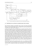
in detail, since it is the simplest one. Finally, Section 6.5 illustrates the performance of the MRAC
based speed estimator within a sensorless vector controlled induction motor drive.
6.2. SPEED ESTIMATION FROM STATOR CURRENT SPECTRUM
Good feature of all the methods that belong to this group is that speed estimation is not affected by

variation of the machine’s electrical parameters. On the other hand, the most serious shortcoming of
these methods is the need for extensive signal processing, since in general Fast Fourier Transform (FFT)
has to be executed on-line. This at the same time reduces the accuracy of speed estimation during rapid
transients.
Stator current harmonics arising from rotor mechanical and magnetic saliencies, such as rotor slotting,
rotor eccentricity and magnetic saturation, are speed dependent. They are independent of time-varying
machine parameters and exist at any non-zero speed. Digital signal processing and spectral estimation
techniques have made it possible to extract these harmonics with minimal data collection and processing
time. Therefore, the slip frequency and rotor speed of the machine can be estimated by utilising, for
example the rotor slot harmonics, monitored from the stator currents.
Many schemes which employ certain harmonics for slip frequency and rotor speed estimation have been
reported. These methods can be divided into two major groups:
1)
those that use the fundamental excitation to estimate the rotor speed, and
2)
those that use a separate excitation signal from the fundamental excitation to estimate the
rotor speed.
Only one method that belongs to the first group, speed estimation on the basis of rotor slot harmonics, is
discussed in what follows. The rotor slot harmonics can be detected by using monitored stator currents
or stator voltages. As monitoring of stator currents is always required anyway, detection of rotor slot
harmonics by using stator currents is preferred, so that voltage monitoring can be avoided.
A speed estimation scheme that uses FFT technique to extract information regarding rotor slot
harmonics has been proposed for the first time in 1992. Presence of rotor slotting causes existence of
certain harmonics in the stator current spectrum. By performing the FFT of the stator current, one is
capable of extracting the frequency information related to the slot harmonics, so that estimation of the
rotor speed becomes possible. Speed is estimated by decomposition of stator current signal into its
harmonic components to determine the speed dependent slot harmonic frequency, f
sh
, and the machine
fundamental frequency f

e
.
The basic principle of this scheme is as follows. For a given supply frequency f
e
, the speed of the
fundamental rotating field is constant and is the synchronous speed. It is given in revolutions per minute
(rpm) by the well-known equation:
n
f
P
e
e
=
60
(6.1)
where n
e
is the synchronous speed and P is the number of pole pairs. The slip, s, is the difference
between the actual speed n and the synchronous speed n
e
. It is often expressed as a fraction of the
synchronous speed as:
s
nn
n
e
e
=
−
(6.2)

HIGH PERFORMANCE DRIVES
---------------------------------------------------------------------------------------------------------------------------------------
 E Levi, 2001
102
It follows that
n=(1-s)n
e
(6.3)
and
f=(1-s)f
e
(6.4)
Angular frequency of slot harmonics is given with:
ωωω
sh e
Z
P
=±
(6.5)
where Z is the number of rotor slots. Note that the number of rotor slots is normally not known and this
is one of the serious drawbacks of this method. In order to implement the method, it is necessary to
somehow at first acquire the information regarding the number of rotor slots.
Using (6.1) to (6.5), the rotor speed n in rpm is expressed and calculated by the following expression:
n
Z
ff
sh e
=±
60
()

(6.6)
where fundamental harmonic frequency is obtained from the FFT analysis as well. The scheme can
operate quite satisfactorily in a wide speed range, down to 2 Hz. The rotor slot harmonic signal is
however nowadays regarded as insufficient in bandwidth as speed feedback signal in a high performance
drive.
Apart from rotor slot harmonics, numerous other parasitic effects can be utilised for extraction of the
speed estimate from the stator current spectrum. These include rotor mechanical eccentricities, existing
magnetic saliencies, and even deliberately introduced rotor asymmetries. These will not be discussed in
more detail, since their industrial relevance at present is limited.
6.3. OPEN LOOP SPEED ESTIMATION USING INDUCTION MACHINE MODEL ONLY
In the context of speed estimation based on an induction machine model, the term ‘open loop speed
estimation’ means that the speed estimation purely relies on the equations of an induction machine
model. In other words, a corrective action within the speed estimator is not present. If there is certain
corrective action within the model based speed estimator, such an estimator is termed ‘closed loop speed
estimator’ (see next Section). Note that the meaning of ‘open loop’ and ‘closed loop’ in this context is
not in any way related to the speed control loop of the drive - this loop is always closed and that is
precisely the reason why the speed is estimated in the first place.
The first attempt to operate the induction machine with closed loop speed control but without using a
speed sensor was based on an analogue slip calculator that computed the slip frequency and dates back
to 1975. The slip frequency is the difference between the stator frequency and the electrical frequency
corresponding to rotor speed. By calculation of the slip frequency, the speed of the rotor can be
determined. The slip information is obtained by measuring the electrical quantities applied to the
machine. By performing simple signal processing operations on the measured quantities, an analogue
signal proportional to the slip level is derived and used to control the machine. This scheme is applicable
only in steady-state, in a limited speed range, and is therefore inappropriate for high performance vector
control.
During the last couple of years, several open-loop rotor speed estimation methods were developed for
sensorless vector control of induction machine. Calculation of the rotor speed is based on the induction
machine dynamic model. Rotor speed is calculated as the difference between the machine’s synchronous
electrical angular speed and the angular slip frequency. In other words,

ω ω ω
=−
rsl
(6.7)
HIGH PERFORMANCE DRIVES
---------------------------------------------------------------------------------------------------------------------------------------
 E Levi, 2001
103
where
ω
is the rotor speed,
ω
r
is the speed of rotor flux and
ω
sl
is the angular slip frequency. In a rotor
flux oriented controlled induction machine, it is possible to obtain the angular slip frequency by using
the rotor voltage equation of the machine in the rotor flux oriented reference frame. The angular slip
frequency can be calculated from:
ω
ψ
sl
m
r
qs
r
L
T
i

=
(6.8)
where i
qs
can be obtained from the torque equation as:
i
T
P
L
L
qs
er
mr
=
2
3
ψ
(6.9)
Substitution of equation (6.9) into (6.8), considering that
ψ
r
=
ψ
dr
in the rotor flux oriented reference
frame and that
TP
L
L
ii

e
m
r
rs rs
=−
3
2
()
ψψ
αβ βα
(6.10)
yields
()
ω
ψ
ψψ
αβ βα
sl
m
r
r
rs rs
L
T
ii=−
1
2
(6.11)
The electrical angle
φ

r
of the rotor flux vector is defined as:
φ
ψ
ψ
β
α
r
r
r
=
æ
è
ç
ö
ø
÷
−
tan
1
(6.12)
The derivative of the angle equation (6.12) can be used to obtain the electrical angular speed of the rotor
flux. Therefore,
ω
φ
ψ
ψ
ψ
ψ
ψψ

α
β
β
α
αβ
r
r
r
r
r
r
rr
d
dt
d
dt
d
dt
==
−
+
22
(6.13)
If the rotor flux components are known, the electrical angular speed of rotor flux can be calculated by
using equation (6.13). It is convenient to estimate the rotor flux components from the stator voltage
equations. Derivatives of the rotor flux components can be then given as:
d
dt
L
L

vRi L
di
dt
d
dt
L
L
vRi L
di
dt
rr
m
sss s
s
r
r
m
sss s
s
ψ
σ
ψ
σ
α
αα
α
β
ββ
β
=−−

æ
è
ç
ö
ø
÷
=−−
æ
è
ç
ö
ø
÷
(6.14)
Hence
()
[]
()
[]
ψσ
ψσ
ψψψ
αααα
ββββ
αβ
r
r
m
sss ss
r

r
m
sss ss
rrr
L
L
vRidtLi
L
L
vRidtLi
=−−
=−−
=+
ò
ò
22
(6.15)
HIGH PERFORMANCE DRIVES
---------------------------------------------------------------------------------------------------------------------------------------
 E Levi, 2001
104
Electrical angular speed of rotor flux, given with (6.13), and angular slip frequency (6.11) are thus
calculated using (6.14)-(6.15) and measured stator voltages and currents. Finally, the rotor speed is
estimated from:
()
ωω ω
ψ
ψ
ψ
ψ

ψψ ψ
ψψ
α
β
β
α
αβ
αβ βα
=− =
−
+
−−
rsl
r
r
r
r
rr
m
rr
rs rs
d
dt
d
dt
L
T
ii
22 2
1

(6.16)
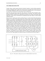
Figure 6.1 shows the diagram of implementation of the speed estimation scheme based on the equations
given above. The inputs are stator currents and stator voltages in stationary reference frame. Stator
currents can be measured from the machine terminals. Stator voltages can be measured from the
machine terminals or reconstructed from the inverter switching states and measured DC link voltage.
Summarising the described procedure, the following equations are utilised:
d
dt
L
L
vRi L
di
dt
d
dt
L
L
vRi L
di
dt
rr
m
sss s
s
r
r
m
sss s
s
ψ

σ
ψ
σ
α
αα
α
β
ββ
β
=−−
æ
è
ç
ö
ø
÷
=−−
æ
è
ç
ö
ø
÷
()
[]
()
[]
ψσ
ψσ
ψψψ

αααα
ββββ
αβ
r
r
m
sss ss
r
r
m
sss ss
rrr
L
L
vRidtLi
L
L
vRidtLi
=−−
=−−
=+
ò
ò
22
(6.17)
()
ωω ω
ψ
ψ
ψ

ψ
ψψ ψ
ψψ
α
β
β
α
αβ
αβ βα
=− =
−
+
−−
rsl
r
r
r
r
rr
m
rr
rs rs
d
dt
d
dt
L
T
ii
22 2

1
Note that all the quantities in (6.17) are in stationary reference frame (that is, alfa-beta components).
Stator current and voltage alfa-beta components are obtained directly from measured phase currents and
voltages, using constant parameter ‘3/2’ transformation (that does not require any angle) of (3.19) and
(3.24).
The problems encountered in the implementation of this scheme are two-fold. Firstly, since it is model
based, accuracy of speed estimation is affected by parameter variation effects. Secondly, the scheme
involves pure integration that fails at very low and zero frequency due to offset and drift problems. This
kind of speed estimator works without failure above 10% of rated synchronous speed.
An alternative speed estimation method is again based on the induction machine voltage equations and
the flux equations in stationary reference frame. The rotor speed can be calculated directly using these
equations. From the machine voltage equations and flux equations the rotor current components in
stationary reference can be expressed as a function of the stator flux:
()
()
i
L
Li
i
L
Li
r
m
sss
r
m
sss
ααα
βββ
ψ

ψ
=−
=−
1
1
(6.18)