idrisi selva tutorial

IDRISI Selva
Tutorial
Manual Version 17
January 2012
J. Ronald Eastman
www.clarklabs.org
IDRISI Source Code
© 1987-2012
IDRISI Production
© 1987-2012
Clark University
J. Ronald Eastman

Introduction 2
Introduction
The exercises of the Tutorial are arranged in a manner that provides a structured approach to the understanding of GIS,
Image Processing, and the other geographic analysis techniques the IDRISI system provides. The exercises are organized
as follows:
Using IDRISI Exercises
Exercises in this section introduce the fundamental terminology and operations of the IDRISI system, including setting
user preferences, display and map composition, and working with databases in Database Workshop.
Introductory GIS Exercises
This set of exercises provides an introduction to the most fundamental raster GIS analytical tools. Using case studies, the
tutorials explore database query, distance and context operators, map algebra, and the use of cartographic models and
IDRISI’s graphic modeling environment Macro Modeler to organize analyses. The final exercises in this section explore
multi-criteria and multi-objective decision making and the use of the Decision Wizard in IDRISI.
Advanced GIS Exercises
Exercises in this section illustrate a range of the possibilities for advanced GIS analysis using IDRISI. These include
regression modeling, predictive modeling using Markov Chain analysis, database uncertainty and decision risk, geostatis-
tics and soil loss modeling with RUSLE.
Introductory Image Processing Exercises

This set of exercises steps the user through the fundamental processes of satellite image classification, using both super-
vised and unsupervised techniques.
Advanced Image Processing Exercises
In this section, the techniques explored in the previous set of exercises are expanded to include issues of classification
uncertainty and mixed-pixel classification. IDRISI provides a suite of tools for advanced image processing and this set of
exercises highlights their use. The final exercise focuses on vegetation indices.
Land Change Modeler Exercises
This set of exercises explores IDRISI’s Land Change Modeler, an integrated vertical application for analyzing past land
cover change, modeling the potential for change, predicting the course of change into the future, assessing the implica-
tions of that change for biodiversity, and evaluating planning interventions for maintaining ecological sustainability.
Earth Trends Modeler Exercises
This set of exercises explores the Earth Trends Modeler, another vertical application within IDRISI for the analysis of
image time series. The Earth Trends Modeler includes a coordinated suite of data mining tools for the extraction of trends
and underlying determinants of variability.
Database Development Exercises
The final section of the Tutorial offers three exercises on database development issues. Resampling and projecting data
are illustrated and some commonly available data layers are imported.
We recommend you complete the exercises in the order in which they are presented within each section, though this is not
strictly necessary. Knowledge of concepts presented in earlier exercises, however, is assumed in subsequent exercises. All
users who are not familiar with the IDRISI system should complete the first set of exercises entitled Using IDRISI. After
this, a user new to GIS and Image Processing might wish to complete the Introductory GIS and Image Processing exer-
cise sections, then come back to the Advanced exercises at a later time. Users familiar with the system should be able to
proceed directly to the particular exercises of interest. In only a few cases are results from one exercise used in a later exer-
cise.
Introduction 3
As you are working on these exercises, you will want to access the Program Modules section in the on-line Help System
any time you encounter a new module. You may also wish to refer to the Glossary section for definitions of unfamiliar
terms.
When action is required at the computer, the section in the exercise is designated by a letter. Throughout most exercises,
numbered questions will also appear. These questions provide opportunity for reflection and self-assessment on the con-

cepts just presented or operations just performed. The answers to these questions appear at the end of each exercise.
When working through an exercise, examine every result (even intermediate ones) by displaying it. If the result is not as
expected, stop and rethink what you have done. Geographical analysis can be likened to a cascade of operations, each one
depending upon the previous one. As a result, there are endless blind alleys, much like in an adventure game. In addition,
errors accumulate rapidly. Your best insurance against this is to think carefully about the result you expect and examine
every product to see if it matches expectations.
Data for the Tutorial are installed in a set of folders, one for each Tutorial section as outlined above. The default installa-
tion folder for the data is given on the first page of each section.
As with all IDRISI documentation, we welcome your comments and suggestions for improvement of the Tutorial.
Tutorial Part 1: Using IDRISI 4
Tutorial Part 1: Using IDRISI
Using IDRISI Exercises
The IDRISI Environment
Display: Layers and Group Files
Display : Layer Interaction Effects
Display : Surfaces Fly Through and Illumination
Display: Navigating Map Query
Map Composition
Palettes, Symbols, and Creating Text Layers
Data Structures and Scaling
Database Workshop: Working with Vector Layers
Database Workshop: Analysis and SQL
Database Workshop : Creating Text Layers / Layer Visibility
Data for the exercises in this section are installed (by default—this may be customized during program installation) to a
folder called \IDRISI Tutorial\Using IDRISI on the same drive as the IDRISI program folder was installed.
Exercise 1-1 The IDRISI Environment 5
Exercise 1-1
The IDRISI Environment
Getting Started
a) To start IDRISI, double-click on the IDRISI application icon in the IDRISI Selva Program Folder. This will

load the IDRISI system.
Once the system has loaded, notice that the screen has four distinct components. At the top, we have the main
menu. Underneath we find the tool bar of icons that can be used to control the display and access commonly
used facilities. Below this is the main workspace, followed by the status bar.
Depending upon your Windows setup, you may also have a Windows task bar at the very bottom of the screen.
If the screen resolution of your computer is somewhat low (e.g., 1024 x 768), you may wish to change your task
bar settings to autohide.
1
This will give you extra space for display—always an essential commodity with a GIS.
Now move your mouse over the tool bar icons. Notice that a short text label pops up below each icon to tell you
its function. This is called a hint. Several other features of the IDRISI interface also incorporate hints.
IDRISI Explorer
b) Click on the File menu and choose the IDRISI Explorer option. This option will launch the IDRISI Explorer
utility. Note that you can also access this same module by clicking the left-most tool bar icon.
IDRISI Explorer is a general purpose utility to manage and explore IDRISI files and projects. Use IDRISI Explorer to set
your project environment, manage your group files, review metadata, display files, and simply organize your data with
such tools as copy, delete, rename, and move commands. You can use IDRISI Explorer to view the structure of IDRISI
file formats and to drag and drop files into IDRISI dialog boxes. IDRISI Explorer is permanently docked to the left edge
of the IDRISI desktop. It can not be moved but it can be minimized and horizontally resized whenever more workspace
is required. We will explore the various uses of IDRISI Explorer in the exercises that follow.
Projects
c) With IDRISI Explorer open, select the Projects tab at the top of IDRISI Explorer. This option allows you to set
the project environment of your file folders. Make sure that the Editor pane is open at the bottom of the Proj-
ects’ tab. If you right-click anywhere in the Projects form you will have the option to show the Editor. The Edi-
tor pane will show the working and resource folders for each project .
During the installation a “Default” project is created. Make sure that you have selected this project by clicking on
1. This can be done from the START menu of Windows. Choose START, then SETTINGS, then Task bar. Click "always on top" off and "autohide" on.
When you do this, you simply need to move your cursor to the bottom of the screen in order to make the task bar visible.
Exercise 1-1 The IDRISI Environment 6
it. The result will have the radio button highlighed for that project.

A project is an organization of data files, both the input files you will use and the output files you will create. The most
fundamental element is the Working Folder. The Working Folder is the location where you will typically find most of your
input data and will write most of the results of your analyses.
2
The first time IDRISI is launched, the Working Folder by
default is named:
\\IDRISI Tutorial Data\Using IDRISI
d) If it is not set this way already, change the Working Folder to be the Using
IDRISI folder.
3
To change the Working Folder, click in the Working Folder
input box and either type in the location or select the browse button to the
right to locate the Using IDRISI folder.
In addition to the Working Folder, you can also have any number of Resource
Folders. A Resource Folder is any folder from which you can read data, but to
which you typically will not write data.
For this exercise, define one Resource Folder:
\\IDRISI Tutorial Data\Introductory GIS
If this is not correctly set, use the New Folder icon at the bottom of the Edi-
tor pane to specify the correct Resource Folder. Note that to remove folders,
you must highlight them in the list first and then click the Remove Folder
icon at the bottom of Editor.
e) The project should now show \\IDRISI Tutorial Data\Using IDRISI as the
Working Folder and \\IDRISI Tutorial Data\Introductory GIS as the
Resource Folder. Your settings are automatically saved in a file named
DEFAULT.ENV (the .env extension stands for Project Environment File).
As new projects are created, you can always use Projects in IDRISI Explorer
to re-load these settings.
IDRISI maintains your Project settings from one session to the next. Thus
they will change only if they are intentionally altered. As a consequence, there

is no need to explicitly save your Project settings unless you expect to use
several projects and wish to have a quick way of alternating between them.
f) Now click the Files tab in IDRISI Explorer. You are now ready to start
exploring the IDRISI system. We will discuss IDRISI Explorer more in
depth later, but from the Files tab you will see a list of all files in your working and resource folders.
The data for the exercises are installed in several folders. The introduction to each section of the Tutorial indicates which
particular folder you will need to access. Whenever you begin a new Tutorial section, change your project accordingly.
2. You can always specify a different input or output path by typing that full path in the filename box directly or by using the Browse button and select-
ing another folder.
3. During installation, the default location will be to the Public folder designated by Windows. This will usually be in a shared documents folder in Users
or Documents and Settings. Adjust these instructions accordingly.
Exercise 1-1 The IDRISI Environment 7
A Special Note to Educators
In normal use, the Working Folder is used for both input and output data. However, if multiple students will be using the
same data in a laboratory setting, you may prefer to set the Project as follows:
Working Folder: A temporary folder to hold all student output data.
Resource Folder(s): The folder(s) in which the original tutorial input data are stored.
Note that all the files that comprise raster (.rgf), vector (.vlx), or signature (.sgf) groups must be in the same folder. When
an exercise requires students to add new files from the Working Folder to groups stored in a Resource Folder, they should
first copy all the files to group from the Resource Folder to the Working Folder.
Dialog Boxes and Pick Lists
Each of the menu entries, and many of the tool bar icons, access specific IDRISI modules. A module is an independent
program element that performs a specific operation. Clicking a menu entry thus results in launching a dialog box (or win-
dow) in which you can specify the inputs to that operation and the various options that you wish to use.
g) There are three ways to launch IDRISI module dialog boxes. The most commonly used modules have toolbar
icons. Click the Display icon to launch the DISPLAY Launcher dialog. Close the dialog by clicking the X in the
upper right corner of the dialog window. Now go to the Display menu and click on the DISPLAY Launcher
menu entry. Close the dialog again. Finally, you can access an alphabetical list of all the IDRISI modules with the
Shortcut utility, located at the top of the IDRISI window. Shortcut will stay open until you choose the Turn
Shortcut Off command under the File Menu. Click the dropdown list arrow on Shortcut and scroll down until

you find DISPLAY Launcher, then click on it and click the Open Dialog button (green arrow to the right of
Shortcuts), or simply hit Enter. Note that you may also type the module name directly into the Shortcut box. In
the Tutorial Exercises, you will typically be instructed to find module names in their menu location to reinforce
your knowledge of the way in which a module is being used. The dialog box will be the same, however, no mat-
ter how it has been opened.
h) Notice first the three buttons at the bottom of the DISPLAY Launcher dialog. The OK button is used after all
options have been set and you are ready to have the module do its work. By default IDRISI dialogs are persistent
i.e., the dialog does not disappear when you click OK. It does the work, but stays on the screen with all of its
settings in case you want to do a similar analysis. If you would prefer that dialogs immediately close after clicking
OK, you can go to the User Preferences option under the File menu and disable persistent dialogs. (Note: hav-
ing said this, DISPLAY Launcher is never persistent.)
If persistent dialogs are enabled, the button to the right of the OK button will be labeled as Close. Clicking on
this both closes the dialog and cancels any parameters you may have set. If persistent forms are disabled, this
button will be labeled Cancel. However, the action is the same Cancel always aborts the operation and closes
the dialog.
i) The Help button can be used to access the context-sensitive Help System. You probably noticed that the main
menu also has a Help button. This can be used to access the IDRISI Help System at its most general level. How-
ever, accessing the Help button on a dialog will bring you immediately to the specific Help section for that mod-
ule. Try it now. Then close the Help window by clicking the X button in its upper-right corner.
The Help System does not duplicate information in the manuals. Rather, it is a supplement, acting as the primary technical
reference for specific program modules. In addition to providing directions for the operation of a module and explaining
its options, the Help System also provides many helpful tips and notes on the implementation of these procedures in the
Exercise 1-1 The IDRISI Environment 8
IDRISI system.
Dialogs are primarily made up of standard Windows elements such as input boxes (the white boxes) in which text can be
entered, radio buttons (such as the file type radio button group), check boxes (such as those to indicate whether or not the
map layer should be displayed with a legend), buttons, and so on. However, IDRISI has incorporated some special dialog
elements to facilitate your use of the system.
j) In DISPLAY Launcher, make sure the
File Type indicates that you wish to dis-

play a raster layer. Then click the small
button with the ellipses, just to the right
of the left input box. This will launch the
pick list. IDRISI uses this specially-
designed selection tool throughout the
system.
The pick list displays the names of map layers and
other data elements, organized by folders. Notice
that it lists your Working Folder first, followed by
each Resource Folder. The pick list always opens with the Working Folder expanded and the Resource Folders collapsed.
To expand a collapsed folder, click on the plus sign next to the folder name. To collapse a folder, click on the minus sign
next to the folder name. A listed folder without a plus/minus symbol is an indication that the folder contains no files of
the type required for that particular input box. Note that you can also access other folders using the Browse button.
k) Collapse and expand the two folders. Since the pick list was invoked from an input box requiring the name of a
raster layer, the files listed are all the raster layers in each folder. Now expand the Working Folder. Find the raster
layer named SIERRADEM and click on it. Then click on the OK button of the pick list. Notice how its name is
now entered into the input box on DISPLAY Launcher and the pick list disappears.
4
Note that double-clicking on a layer in the pick list will achieve the same result as above. Also note that double-clicking on
an input box is an alternate way of launching the pick list.
l) Now that we have selected the layer to be displayed, we need to choose an appropriate palette (a sequence of
colors used in rendering the raster image). In most cases, you will use one of the standard palettes represented by
radio buttons. However, you will learn later that it is possible to create a virtually infinite number of palettes. In
this instance, the IDRISI Default Quantitative palette is selected by default and is the palette we wish to use.
m) Notice that the autoscale option has been automatically set to Equal Intervals by the display system. This will be
explained in greater detail in a later exercise. However, for now it is sufficient to know that autoscaling is a pro-
cedure by which the system determines the correspondence between numeric values in your image (SIERRA-
DEM) and the color symbols in your palette.
n) The legend and title check boxes are self-explanatory. For this illustration, be sure that these check boxes are also
selected and then click OK. The image will then appear on the screen.

This image is a Digital Elevation Model (DEM) of an area in Spain.
4. Note that when input filenames are chosen from the Pick List or typed without a full path, IDRISI first looks for the file in the Working Folder, then
in each Resource Folder until the file is found. Thus, if files with the same name exist in both the Working and Resource Folders, the file in the Working
Folder will be selected.
Exercise 1-1 The IDRISI Environment 9
The Status and Tool Bars
The Status Bar at the bottom of the screen is primarily used to provide information about a map window.
o) Move the mouse over the map window you just launched. Notice how the status bar continuously updates the
column and row position as well as the X and Y coordinate position of the mouse. Also notice what happens
when the mouse is moved off of the map window.
All map layers will display the X and Y positions of the mouse—coordinates representing the ground position in a spe-
cific geographic reference system (such as the Universal Transverse Mercator system in this case). However, only raster
layers indicate a column and row reference (as will be discussed further below).
Also note the Representative Fraction (RF) on the left of the status bar. The RF expresses the current map scale (as seen
on the screen) as a fraction reduction of the true earth. For example, an RF = 1/5000 indicates that the map display
shows the earth 5000 times smaller than it actually is.
p) Like the position fields, the RF field is updated continuously. To get a sense of this, click the icon marked Full
Extent Maximized (pause the cursor over the icons to see their names). Notice how the RF changes. Then click
the Full Extent Normal icon. These functions are also activated by the End and Home keys. Press the End key
and then the Home key.
You can set a specific RF by right-clicking in image. Select Set specific RF from the menu. A dialog will allow
you to set a specific RF. Clicking OK will display the image at this specified scale.
As indicated earlier, many of the tool bar icons launch module dialogs, just like the menu system. However, some of them
are specifically designed to access interactive features of the display system, such as the two you just explored. Two other
interactive icons are the Measure tools, both length and zone.
q) Click on the Measure Length icon located near the center of the top icons and represented by a ruler. Then,
move the cursor into the SIERRADEM image and left-click to begin measuring a length. As you move the cur-
sor in any direction, an accompanying dialog will record the length and azimuth along the length of the line. If
you continue to left-click, you can add additional segments that will add length to the original segment. A right-
click of the mouse will end measuring.

Click on the Measure Zone icon located to the right of the Measure Length icon. Then click anywhere in the
image and move the mouse. As you drag the mouse, a circle will be drawn with a dialog showing the radius and
area of the circle. A right-click will end this process.
Menu Organization
As distributed, the main menu has nine sections: File, Display, GIS Analysis, Modeling, Image Processing, Reformat, Data
Entry, Window List, and Help. Collectively, they provide access to over 200 analytical modules, as well as a host of special-
ized utilities. The Display, Data Entry, Window List and Help menus are self-evident in their intent. However, the others
deserve some explanation.
As the name suggests, the File menu contains a series of utilities for the import, export and organization of data files.
However, as is traditional with Windows software, the File menu is also where you set user preferences.
r) Open the User Preferences dialog from the File menu. We will discuss many of these option later. For now, click
on the Display Settings tab and then the Revert to Defaults button to ensure that your settings are set properly
for this exercise. Click OK.
Exercise 1-1 The IDRISI Environment 10
The Reformat menu contains a series of modules for the purpose of converting data from one format to another. It is
here, for example, that one finds routines for converting between raster and vector formats, changing the projection and
grid reference system of map layers, generalizing spatial data and extracting subsets.
The GIS Analysis and Image Processing menus contain the majority of modules. The GIS Analysis menu is two to four
levels deep, with its primary organization at level two. The first four menu entries at this second level represent the core of
GIS analysis: Database Query, Mathematical Operators, Distance Operators and Context Operators. The others represent
major analytical areas: Statistics, Decision Support, Change and Time Series Analysis, and Surface Analysis. The Image
Processing menu includes ten submenus.
The Modeling menu includes tools and facilities for constructing models as well as information for calling IDRISI capa-
bilities from user-written programs.
s) Go to the Surface Analysis submenu under the GIS Analysis main menu and explore the four submenus there.
Note that most of the menu entries that open module dialog boxes (i.e., the end members of the menu trees) are
indicated with capital letters but some are not. Those designated with capital letters can be used as procedures
with the IDRISI Macro Language (IML). Now click on the CONTOUR menu entry in the Feature Extraction
submenu to launch the CONTOUR module.
t) From the CONTOUR dialog, specify SIERRADEM as the input raster image. (Recall that the pick list may be

launched with the Pick List button, or by double-clicking on the input box.)
Enter the name CONTOURS as the output vector file. For output files, you cannot invoke the pick list to
choose the filename because we are creating a new file. (For output filename boxes, the pick list button allows
you to direct the output to a folder other than the Working Folder. You also can see a list of filenames already
present in the Working Folder.)
Change the input boxes to specify a minimum contour value of 400 and a maximum of 2000, with a contour
interval of 100. You can leave the default values for the other two options. Enter a descriptive title to be
recorded in the documentation of the output file. In this case, the title "100 m Contours from SIERRADEM"
would be appropriate. Click OK. Note that the status bar shows the progress of this module as it creates the
contours in two passes—an initial pass to create the basic contours and a second pass to generalize them. When
the CONTOUR module has finished, IDRISI will automatically display the result.
The automatic display of analytical results is an optional feature of the System Settings of the User Preferences dialog
(under the File menu). The procedures for changing the Display Settings will be covered in the next exercise.
u) Move your cursor over the CONTOURS map window. Note that it does not display a column and row value in
the status bar. This is because CONTOURS is a vector layer.
Composer and Navigation
v) To appreciate the difference between raster and vector layers better, close the CONTOURS map window by
clicking on the X button on its upper-right corner. Then, with the SIERRADEM display active, click the Add
Layer option of the Composer dialog and specify CONTOURS as the vector layer and Outline Black as the sym-
bol file. Click OK to add this layer to your composition.
Composer is one of the most important tools you will use in the construction of map compositions. It allows
you to add and remove layers, change their hierarchical position and symbolization, and ultimately save and print
map compositions. Composer will be explored in far greater depth in the next exercise. By default, Composer
will always be displayed on the right-side of the desktop when any map window is open.
Exercise 1-1 The IDRISI Environment 11
w) Along with Composer, the navigation tools on the tool bar (which are also available on the keyboard and mouse)
are essential for manipulating the map window. The tool bar has several icons for navigating around a map layer.
There are icons for panning, zooming and changing the size or extent of the map window. These functions are
dupliated by keyboard and mouse operations. The zoom in and zoom out icons not only zoom, but also center
the image depending on where you place your cursor. The PgUp and PgDn keys on the keyboard are similar but

without the recentering. The Full Extent Normal and Full Extent Maximized icons are duplicated by the Home
and End keys. With the keyboard you can also pan using the arrow keys and with a properly supported mouse,
you can zoom in and out using the mouse wheel.
Now pan to an area of interest and zoom in until the cell structure of the raster image (SIERRADEM) becomes
evident. As you can see, the raster image is made up of a fine cellular structure of data elements (that only
become evident under considerable magnification). These cells are often referred to as pixels. Note, however,
that at the same scale at which the raster structure becomes evident, the vector contours still appear as thin lines.
In this instance, it would seem that the vector layer has a higher resolution, but looks can be deceiving. After all, the vector
layer was derived from the raster layer. In part, the continuity of the connected points that make up the vector lines gives
this impression of higher resolution. The generalization stage also served to add many additional interpolated points to
produce the smooth appearance of the contours. The chapter Introduction to GIS in the IDRISI Manual discusses ras-
ter and vector GIS data structures.
Alternative Graphic Displays
The construction of map compositions through the use of DISPLAY Launcher and Composer will represent one of the
most important tools you will use in GIS. These will be explored in much further depth in the following exercise. How-
ever, IDRISI provides a variety of other means for viewing geographic data. To finish off this exercise, we will explore the
ORTHO module which provides one of two facilities within IDRISI for creating three-dimensional displays.
x) Click on the DISPLAY Launcher icon and specify the raster layer named SIERRA234. Note that the palette
options are disabled in this instance because the image represents a 24-bit full color image
5
(in this case, a satel-
lite image created from bands 2, 3 and 4 of a Landsat scene). Click OK.
y) Now choose the ORTHO option from the DISPLAY menu. Specify SIERRADEM as the surface image and
SIERRA234 as the drape image. Since this is a 24-bit image, you will not need to specify a palette. Keep the
default settings for all other parameters except for the output resolution. Choose one level below your display
system's resolution.
6
For example, if your system displays images at 1024 x 768, choose 800 x 600. Then click
OK. When the map window appears, press the End key to maximize the display.
5. A 24-bit image is a special form of raster image that contains the data for three independent color channels which are assigned to the red, green and

blue primaries of the display system. Each of these three channels is represented by 256 levels, leading to over 16 million displayable colors. However,
the ability of your system to resolve this image will depend upon your graphics system. This can easily be determined by minimizing IDRISI and clicking
the right mouse button on the Windows desktop. Then choose the Settings tab of the Display Properties dialog. If your system is set for 24-bit true color,
you are seeing this image at its fullest color resolution. However, it is as likely as not that you are seeing this image at some lower resolution. High color
settings (15 or 16 bit) look almost indistinguishable from 24-bit displays, but use far less memory (thus typically allowing a higher spatial resolution).
However, 256 color settings provide quite poor approximations. Depending upon your system, you will probably have a choice of settings in which you
trade off color resolution for spatial resolution. Ideally, you should choose a 24-bit true color or 16-bit high color option and the largest spatial resolu-
tion available. A minimum of 800 x 600 spatial resolution is recommended, but 1024 x 768 or better is more desirable.
6. If you find that the resulting display has gaps that you find undesirable, choose a lower resolution. In most instances, you will want to choose the
highest resolution that produces a continuous display. The size of the images used with ORTHO (number of columns and rows) influences the result, so
in one case, the best result may be obtained with one resolution, while with another dataset, a different resolution is required.
Exercise 1-1 The IDRISI Environment 12
The three-dimensional (i.e., orthographic) perspective offered through ORTHO can produce extremely dramatic displays
and is a powerful tool for visual analysis. Later we will explore another module that not only produces three dimensional
displays, but also allows you to fly through the model!
The rest of the exercises in this section of the Tutorial focus primarily on the elements of the Display System.
Housekeeping
As you are probably now beginning to appreciate, it takes little time before your workspace is filled with many windows.
Go to the Window List menu. Here you will find a list of all open dialogs and map windows. Clicking on any of these will
cause that window to come to the top. In addition, note that you can close groups of open windows from this menu.
Choose Close All Windows to clean off the screen for the next exercise.
Exercise 1-2 Display: Layers and Group Files 13
Exercise 1-2
Display: Layers and Group Files
The digital representation of spatial data requires a series of constituent elements, the most important of which is the map
layer. A layer is a basic geographic theme, consisting of a set of similar features. Examples of layers include a roads layer, a
rivers layer, a landuse layer, a census tract layer, and so on. Features are the constituents of map layers, and are the most
fundamental geographic entities—the equivalent of molecules, which are in turn compounds of more basic atomic fea-
tures such as nodes, vertices and lines.
At a higher level, layers can be understood to be the basic building blocks of maps. Thus a map might be composed of a

state boundaries layer, a forest lands layer, a streams layer, a contours layer and a roads layer, along with a variety of ancil-
lary map components such as legends, titles, a scale bar, north arrow, and the like.
With traditional geographic representations, the map is the only entity that we can interact with. However, in GIS, any of
these levels are available to us. We can focus the display on specific features, isolated layers, or we can view any of a series
of multi-layer custom-designed maps. It is the layer, however, that is unquestionably the most important of these. Layers
are not only the basic building blocks of maps, but they are also the basic elements of geographic analysis. They are the
variables of geographic models. Thus our exploration of GIS logically starts with map layers, and the display system that
allows us to explore them with the most important analytical tool at our disposal—the visual system.
Displaying Map Layers
Since the earliest days of automated cartography and GIS, map layers have been digitally encoded according to two funda-
mentally different logics—raster and vector. The fact that both formats are still very much in use attests to the fact that each
has special strengths. Indeed, most GIS software systems, including IDRISI, have moved towards the integration of the
two. Thus, as you work with the system, you will work with both forms of representation.
a) Make sure your main Working Folder is set to Using IDRISI. Then click on the DISPLAY Launcher icon on the
tool bar. Note that separate options are included for raster and vector layers, as well as a map composition
option (which we will explore in a later exercise). Despite the fact that their representational structures are very
different, your means of displaying and interacting with them is identical.
Display the vector layer named SIERRAFOREST. Select the user-defined symbol option, invoke the pick list for
the symbol files and choose the symbol file Forest. Turn the title and legend options off. Click OK.
This is a vector layer of forest stands for the Sierra de Gredos area of Spain. We examined a DEM and color
composite image of this area in the previous exercise. Vector layers are composed of points, which are linked to
form lines and areal boundaries of polygons.
7
Use the zoom (PgUp and PgDn) and pan keys (the arrows) to
focus in on some of these forest polygons. If you zoom in far enough, the vector structure should become
quickly apparent.
b) Press the Home key to restore the original display and then the End key to maximize the display of the layer.
7. Areal features, such as provinces, are commonly called polygons because the points which define their boundaries are always joined by straight lines,
thus producing a multi-sided figure. If the points are close enough, a linear or polygonal feature will appear to have a smooth boundary. However, this is
only a visual appearance.

Exercise 1-2 Display: Layers and Group Files 14
Now select the Cursor Inquiry Mode icon on the toolbar (the icon with the question mark and arrow). When
you move the cursor into the map display, notice that it changes to a cross-hair. Click on a forest polygon. The
polygon becomes highlighted and its ID is shown near the cursor. Click on several other forest polygons. Also
click on some of the white areas between these polygons. Then open the Feature Properties box by clicking on
the Feature Properties tool bar icon to the immediate right of the Cursor Inquiry Mode icon, and continue to
click on polygons. Note the information presented in the Feature Properties box that opens below Composer.
What should be evident here is that vector representations are feature-oriented—they describe features—entities with dis-
tinct boundaries—and there is nothing between these features (the void!). Contrast this with raster layers.
c) Click on the Add Layer button on Composer. This dialog is a modified version of DISPLAY Launcher with
options to add either an additional raster or vector layer to the current composition. Any number of layers can
be added in this way. In this instance, select the raster layer option and choose SIERRANDVI from the pick list
options. Then choose the NDVI palette and click OK.
This is a vegetation biomass image, created from satellite imagery using a simple mathematical model.
8
With this
palette, greener areas have greater biomass. Areas with progressively less biomass range from yellow to brown to
red. This is primarily a sparse dry forest area.
d) Notice how this raster layer has completely covered over the vector layer. This is because it is on top and it con-
tains no empty space. To confirm that both layers are actually there, click on the check mark beside the SIER-
RANDVI layer in the Composer dialog. This will temporarily turn its visibility off, allowing you to see the layer
below it.
Make the raster layer visible again by clicking to the left of the filename. Raster layers are composed of a very
fine matrix of cells commonly called pixels,
9
stored as a matrix of numeric values, but represented as a dense grid
of varying colored rectangles.
10
Zoom in with the PgDn key until this raster structure becomes apparent.
Raster layers do not describe features in space, but rather the fabric of space itself. Each cell describes the condi-

tion or character of space at that location, and every cell is described. Since Cursor Inquiry Mode is still on, first
click on the SIERRANDVI filename on Composer (to select it for inquiry) then click onto a variety of cells with
the cursor. Notice how each and every cell contains a value. Consequently, when a raster layer is in a composi-
tion, we generally cannot see through to any layers below it. Conversely, this is generally not the case with vector.
However, the next exercise will explore ways in which we can blend the information in layers and make back-
ground areas transparent.
e) Change the position of the layers so that the vector layer is on top. To do this, click the name of the vector layer
(SIERRAFOREST) in Composer so that it becomes highlighted. Then press and hold the left mouse button
down over the highlighted bar and drag it until the pointer is over the SIERRANDVI filename and it becomes
highlighted, then release the mouse button. This will change its position.
With the vector layer on top, notice how you can see through to the layer below it wherever there is empty space.
However, the polygons themselves obscure everything behind them. This can be alleviated by using a different
form of symbolization.
8. NDVI and many other vegetation indices are discussed in detail in the chapter Vegetation Indices in the IDRISI Manual as well as Tutorial Exer-
cise 5-7.
9. The word pixel is a contraction of the words picture and element. Technically a pixel is a graphic element, while the data value which underlies it is a grid
cell value. However, in common parlance, it is not unusual to use the word pixel to refer to both.
10. Unlike most raster systems, IDRISI does not assume that all pixels are square. By comparing the number of columns and rows against the coordinate
range in X and Y respectively, it determines their shape automatically, and will display them either as squares or rectangles accordingly.
Exercise 1-2 Display: Layers and Group Files 15
f) Select the SIERRAFOREST layer in Composer. Then click on the Layer Properties button. Layer Properties, as
the name suggests, displays some important details about the selected (highlighted) layer, including the palette or
symbol file in use.
You have two options to change the symbol file used to display the SIERRAFOREST layer. One would be to
click on the pick list button and select a symbol file, as we did the first time. However, in this case, we are going
to use the Advanced Palette/Symbol Selection tool. Click that particular button it is just below the symbol file
input box.
The Advanced Palette/Symbol Selection tool provides quick access to over 1300 palette and symbol files. The
first decision you need to make is whether the data express quantitative variations (such as with the NDVI data),
qualitative differences (such as landcover categories that differ in kind rather than quantity) or simple set mem-

bership depicted with a uniform symbolization. In our case, the latter applies, therefore click on the None (Uni-
form) option. Then select the cross-stripe symbol type (“x stripe”) and a blue color logic. Notice that there are
four blue color options. Any of these four can be selected by clicking on the button that illustrates the color
sequence. Try clicking on these buttons and note what happens in the input box the symbol filename changes!
Thus all you are doing with this interface is selecting symbol files that you could also choose from a pick list.
Ultimately, click on the darkest blue option (the first button on the right) and then click on OK. This returns you
to Layer Properties. You can also click OK here.
Unlike the solid polygon fill of the Forest symbol file, the new symbol file you selected uses a cross-hatch pat-
tern with a clear background. As a result, we can now see the full layer below. In the next exercise you will learn
about other ways of blending or making layers transparent.
From the steps above, we can clearly see that vector and raster layers are different. However, their true relative strengths
are not yet apparent. Over the course of many more exercises, we will learn that raster layers provide the necessary ingre-
dients to a large number of analytical operations—the ability to describe continuous data (such as the continuously vary-
ing biomass levels in the SIERRANDVI image), a simple and predictable structure and surface topology that allows us to
model movements across space, and an architecture that is inherently compatible with that of computer memory. For vec-
tor layers, the real strength of their structure lies in the ability to store and manipulate data for collections of layers that
apply to the features described.
Group Files
In this section, we will begin an exploration of group files. In IDRISI, a group file is a collection of files that are specifi-
cally associated with each other. Group files are associated with raster layers and to signature files. A group file, depending
on the type, will have a specific extension but is always a text file that lists files associated with a group. There are two
types of raster group layers: raster and time series files with .rgf and .ts extensions respectively. Signature group files are of
two types, multispectral signature and hyperspectral signature group files with .sgf and .hgf extensions respectively. All
group files are created using IDRISI Explorer.
Raster Layer Groups
A raster layer group is exactly that—a colletion of raster layers that are grouped together. We will use IDRISI Explorer to
create this group file with a .rgf extension.
g) Open IDRISI Explorer from the File menu. By default IDRISI Explorer opens to the Files tab displaying all the
filtered files in the Working and Resource folders. Like the pick list, you can display files in any of the folders by
scrolling and clicking the appropriate folder name. Make sure you are in the Using IDRISI folder. To create a

raster group file we will select the necessary files and then right-click to create this file.
Exercise 1-2 Display: Layers and Group Files 16
Select each of the following files in turn. You may multi-select files by holding down the shift key to select sev-
eral files listed together or by holding down the control key to select several files individually.
SIERRA1
SIERRA2
SIERRA3
SIERRA4
SIERRA5
SIERRA7
SIERRA234
SIERRA345
SIERRADEM
SIERRANDVI
If you make any mistakes, simply click the file to highlight or remove the
highlight. If it is highlighted, it is selected. Then, right-click in the Files pane
and choose the Create\Raster group option from the menu. By default the
name given to this new group file is RASTER GROUP.RGF. The files con-
tained in the raster group will also be displayed in IDRISI Explorer.
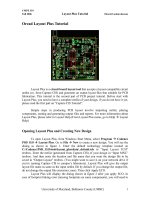
Change the name of the raster group file to SIERRA by right-clicking on
the RASTER GROUP.RGF filename and select Rename.
By default, the Metadata pane should be visible in IDRISI Explorer. If it is
not, right click in the Files pane and select Metadata. Then when you select
the SIERRA group file, Metadata will show the files contained in this group
and their order. In most cases order is not important, but if it is as in the
case of Time Series analysis, you can always change the order in Metadata.
Raster group files provide a range of powerful capabilities, including the ability to
provide tabular summaries about the characteristics of any location.
h) Bring up DISPLAY Launcher and select the raster layer option. Then click
on the pick list button. Notice that your SIERRA group appears with a plus

sign, as well as the individual layers from which it was formed. Click on the
plus sign to list the members of the group and then select the SIERRA345
image. You should now see the text "sierra.sierra345" in the input box.
Since this is a 24-bit composite, you can now click OK without specifying a
palette (this will be explained further in a later exercise). This is a color
composite of Landsat bands 3, 4 and 5 of the Sierra de Gredos area. Leave
it on the screen for the next section.
With raster groups, the individual layers exist independent of the group. Thus, to dis-
play any one of these layers we can specify it either with its direct name (e.g.,
SIERRA345) or with its group name attached (e.g., SIERRA.SIERRA345). What is
the benefit, then, of using a group?
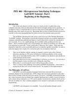
i) We will need to work through several exercises to fully answer this ques-
tion. However, to get a sense, open Feature Properties from the toolbar. Then move the mouse and use the left
mouse button to click on various pixels around the image and look at the Feature Properties box. Next click on
the View as Graph button at the bottom of the Feature Properties box and continue to click on the image.
Cursor Inquiry Mode allows you to inspect the value of any specific pixel. However, with a raster group file, you can
Exercise 1-2 Display: Layers and Group Files 17
examine the values of the whole group at the same pixel location, producing a table or graph as desired.
Displaying Map Layers with IDRISI Explorer
Until this point we have used DISPLAY Launcher to display layers, either individually or as part of a group. Alternatively,
you can display raster and vector files from IDRISI Explorer, simply by double-clicking on the filename from the Files
tab.
j) To display SIERRADEM from IDRISI Explorer, double-click on the filename. The map layer will appear on the
IDRISI Desktop. You can also display a member of a group file by double-clicking on the raster group file to
expose the grouped files, then again double-click on the file to display. The resulting file will be displayed with
the dot logic in the filename, for example, SIERRA.SIERRADEM.
When displaying layers from IDRISI Explorer you will have no control over its initial display characteristics, unlike DIS-
PLAY Launcher. However, once a layer is displayed you can alter its display from Layer Properties in Composer. As we
will see in the next section, IDRISI Explorer can also be used to Add Layers to map compositions, just as in Composer.
Exercise 1-3 Display: Layer Interaction Effects 18

Exercise 1-3
Display: Layer Interaction Effects
As we have seen, map compositions are formed from stacking a series of layers in the same map window using Composer.
By default, the backgrounds of vector layers are transparent while those of raster layers are opaque. Thus, adding a raster
layer to the top of a composition will, by default, obscure the layers below. However, IDRISI provides a number of multi-
layer interaction effects which can modify this action to create some exciting display possibilities.
Blends
a) If your workspace contains any existing windows, clean it off by using the Close All Windows option from the
Window List menu. Then use DISPLAY Launcher to view the image named SIERRADEM using the Default
Quantitative palette. The colours in this image are directly related to the height of the land. However, it does not
convey well the nature of the relief. Therefore we will blend in some hillshading to give a sense of the topogra-
phy.
b) First, go to the Surface Analysis section of the GIS Analysis menu and then the Topographic Variables submenu
to select HILLSHADE. This option accesses the SURFACE module to create hillshading from your digital ele-
vation model. Specify SIERRADEM as the elevation model and SIERRAHS as the output. Leave the sun azi-
muth and elevation values at their default values and simply click OK.
The effect here is clearly dramatic! To create this by hand would have taken the skills of a talented topographer
and many weeks of painstaking artistic rendition using a tool such as an air brush. However, through illumina-
tion modeling in GIS, it takes only moments to create this dramatic rendition.
c) Our next step is to blend this with our digital elevation model. Remove the hillshaded image from the screen by
clicking the X in its upper-right corner. Then click onto the banner of the map window containing SIERRA-
DEM and click Add Layer in Composer. When the Add Layer dialog appears, click on Raster as the layer type
and indicate SIERRAHS as the image to be displayed. For the palette, select Greyscale.
Notice how the hillshaded image obscures the layer below it. We will move the SIERRADEM layer so it is on
top of the hillshading layer by dragging it
11
with the mouse so it is at the bottom position in Composer’s layer
list. At this point, the DEM should be obscuring the hillshading.
Now be sure SIERRADEM is highlighted in Composer (click on its name if it isn’t) and then click the Blend
button on Composer.

The Blend button blends the color information of the selected layer 50/50 with that of the assemblage of visible
elements below it in the map composition. The Layer Properties button contains a visibility dialog that allows
other proportions to be used (such as 60/40, for example). However, a 50% blend is typically just right. Note
that the blend can be removed by clicking the Blend button a second time while that layer is highlighted in Com-
poser. This application is probably the most common use of blend to include topographic hillshading. How-
11. To drag it, place the mouse over the layer name and press and hold the left mouse button down while you move the mouse to the new position
where you want the layer to be. Then release the left mouse button and the move will be implemented.
Exercise 1-3 Display: Layer Interaction Effects 19
ever, any raster layer can be blended.
12

Vector layers cannot be blended directly. However, they can be affected by blends in raster layers visually above
them in the composition. To appreciate this, click the Add Layer button on Composer and specify the vector
layer named CONTOURS that you created in the first exercise. Then click on the Advanced Palette/Symbol
Selection tab. Set the Data Relationship to None (uniform), the Symbol Type to Solid, and the Color Logic to Blue.
Then click on the last choice to select LineSldUniformBlue4 and click OK. As you can see, the contours somewhat
dominate the display. Therefore drag the CONTOURS layer to the position between SIERRAHS and SIERRA-
DEM. Notice how the contours appear in a much more subtle color that varies between contours. The reason
for this is that the color from SIERRADEM has now blended with that of the contours as well.
Before we go on to consider transparency, let’s make the color of SIERRADEM coordinate with the contours.
First be sure that the SIERRADEM layer is highlighted in Composer by clicking onto its name. Then click the
Layer Properties button. In the Display Min/Max Contrast Settings input boxes type 400 for the Display Min
and 2000 for the Display Max. Then change the Number of Classes to 16 and click the Apply button, followed
by OK. Note the change in the legend as well as the relationship between the color classes and the contours.
Keep this composition on the screen for use in the next section.
Transparency
d) Let’s now define the lakes and reservoirs. Although we don’t have direct data for this, we do have the near-infra-
red band from a Landsat image of the region. Near-infrared wavelengths are absorbed very heavily by water.
Thus open water bodies tend to be quite distinctive on near-infrared images. Click onto the DISPLAY Launcher
icon and display the layer named SIERRA4. This is the Landsat Band 4 image. Use Cursor Inquiry to examine

pixel values in the lakes. Note that they appear to have reflectance values less than 30. Therefore it would appear
that we can use this threshold to define open water areas.
e) Click on the RECLASS icon on the toolbar. Set the type of file to be reclassified to Image and the classification
type to User-Defined. Set the input file to SIERRA4 and the output file to LAKES. Set the reclass parameters to
assign:
a 1 to values from 0 to just less than 30, and
a 0 to values from 30 to just less than 999.
Then click on OK. The result should be the lakes and reservoirs we want. However, since we want to add it to
our composition, remove the automatically displayed result.
f) Now use the Add Layer button on Composer to add the raster layer LAKES. Again use the Advanced Palette/
Symbol Selection tab and set the Data Relationship to None (uniform), the Color Logic to Blue and then click the
third choice to select UniformBlue3.
g) Clearly there is a problem here the LAKES layer obscures everything below it. However, this is easily reme-
died. Be sure the LAKES layer is highlighted in Composer and then click the right-most of the small buttons
above Add Layer.
This is the Transparency button. It makes all pixels assigned to color 0 in the prevailing palette transparent
12. Vector layers cannot be the agents of a blend. However, they can be affected by blends in raster layers above them, as will be demonstrated in this
exercise.
Exercise 1-3 Display: Layer Interaction Effects 20
(regardless of what that color is). Note that a layer can be made both transparent and blended try it! As with
the blend effect, clicking the Transparent button a second time while a transparent layer is highlighted will cause
the transparency effect to be removed.
Composites
In the first exercise, you examined a 24-bit color composite layer, SIERRA234. Layers such as this are created with a spe-
cial module named COMPOSITE. However, COMPOSITE images can also be created on the fly through the use of Com-
poser. We will explore both options here.
h) First remove any existing images or dialogs. Then use DISPLAY Launcher to display SIERRA4 using the
Greyscale palette. Then press the “r” key on the keyboard. This is a shortcut that launches the Add Layer dialog
from Composer, set to add a raster layer (note that you can also use the shortcut “v” to bring up Add Layer set
to add a vector layer). Specify SIERRA5 as the layer and again use the Greyscale palette. Then use the “r” short-

cut again to add SIERRA7 using the Greyscale palette. At this point, you should have a map composition con-
taining three images, each obscuring the other.
Notice that the small buttons above Add Layer in Composer include three with red, green and blue colors. Be
sure that SIERRA7 is highlighted in Composer and then click on the Red button. Then highlight SIERRA5 in
Composer (i.e., click onto its name) and then click the Green button. Finally, highlight SIERRA4 in Composer
and click the Blue button.
Any set of three adjacent layers can be formed into a color composite in this way. Note that it was not important
that they had a Greyscale palette to start with any initial palette is fine. In addition, the layers assigned to red,
green and blue can be in any order. Finally, note that as with all of the other buttons in this row on Composer,
clicking it a second time while that layer is highlighted causes the effect to be removed.
Creating composites on the fly is very convenient, but not necessarily very efficient. If you are going to be working with a
particular composite often, it is much easier to merge the three layers into a single 24-bit color composite layer. 24-bit
composite layers have a special data type, known as RGB24 in IDRISI. These are IDRISI’s equivalent of the same kind of
color composite found in BMP, TIFF and JPG files.
Open the COMPOSITE module, either from the Display menu or from its toolbar icon. Here we can create 24-bit com-
posite images. Specify SIERRA4, SIERRA5 and SIERRA7 as the blue, green and red bands, respectively. Call the output
SIERRA457. We will use the default settings to create a 24-bit composite with original values and stretched saturation
points with a default saturation of 1%. Click OK.
The issue of scaling and saturation will be covered in more detail in a later exercise. However, to get a quick sense of it,
create another composite but use a temporary name for the output and use the simple linear option. To create a tempo-
rary output name, simply double-click in the output name box. This will automatically generate a name beginning with the
prefix “tmp” such as TMP000.
Notice how the result is much darker. This is caused by the presence of very bright, isolated features. Most of the image is
occupied by features that are not quite so bright. Using simple linear scaling, the available range of display brightnesses on
each band is linearly applied to cover the entire range, including the very bright areas. Since these isolated bright areas are
typically very small (in many cases, they can’t even be seen), we are sacrificing contrast in the main brightness region in
order to display them. A common form of contrast enhancement, then, is to set the highest display brightness to a lower
scene brightness. This has the effect of saturating the brightest areas (i.e., assigning a range of scene brightnesses to the
same display brightness), with the positive impact that the available display brightnesses are now much more advanta-
geously spread over the main group of scene brightnesses. Note, however, that the data values are not altered by this pro-

cedure (since you used the second option for the output type to create the 24 bit composite using original values with
Exercise 1-3 Display: Layer Interaction Effects 21
stretched saturation points). This procedure only affects the visual display. The nature of this will be explained further in a
later exercise. In addition, note that when you used the interactive on the fly composite procedure, it automatically calcu-
lated the 1% saturation points and stored these as the Display Min and Max values for each layer
13
.
Anaglyphs
Anaglyphs are three-dimensional representations derived from superimposing a pair of separate views of the same scene
in different colors, such as the complementary colors, red and cyan. When viewed with 3-D glasses consisting of a red
lens for one eye and a cyan lens for the other, a three-dimensional view can be seen. To work properly, the two views
(known as stereo images) must possess a left/right orientation, with an alignment parallel to the eye
14
.
i) Use the Close All Windows option of the Window List menu to clear the screen. Then use DISPLAY Launcher
to view the file named IKONOS1 using the Greyscale palette. Then use Add Layer in Composer (or press the
“r” key) to add the image named IKONOS2, again with the Greyscale palette.
Click the checkmark next to the IKONOS2 image in Composer on and off repeatedly. These two images are
portions of two IKONOS satellite images (www.spaceimaging.com) of the same area (San Diego, United States,
Balboa Park area), but they are taken from different positions hence the differences evident as you compare
the two images.
More specifically, they are taken at two positions along the satellite track from north to south (approximately) of
the IKONOS satellite system. Thus the tops of these images face west. They are also epipolar. Epipolar images
are exactly aligned with the path of viewing. When they are viewed such that the left eye only sees the left image
(along track) and the right eye only sees the right image, a three-dimensional view is perceived.
Many different techniques have been devised to present each eye with the appropriate image of a stereo pair. One
of the simplest is the anaglyph. With this technique each image is portrayed in a special color. Using special eye-
glasses with filters of the same color logic on each eye, a three-dimensional image can be perceived.
j) IDRISI can accommodate all anaglyphic color schemes using the layer interaction effects provided by Com-
poser. However, the red/cyan scheme typically provides the highest contrast. First be sure that the IKONOS2

image is highlighted in Composer and is checked to be visible. If it is not, click on its name in Composer. Then
click on the Cyan button of the group above Add Layer (Cyan is the light blue color, also known as aquamarine).
Then highlight the IKONOS1 image and click on the Red button above Add Layer. Then view the result with
the 3-D glasses, such that the red lens is over the left eye and the cyan lens is over the right eye. You should now
see a three-dimensional image. Then try reversing the eye glasses so that the red lens is over the right eye. Notice
how the three dimensional image becomes inverted. In general, if you get the color sequence reversed, you
should always be able to figure this out by looking at what happens with familiar objects.
This is only a small portion of an IKONOS stereo scene. Zoom in and roam around the image. The resolution
is 1 meter truly extraordinary! Note that other sensor systems are also capable of producing stereo images,
including SPOT, QUICKBIRD and ASTER. However, you may need to reorient the images to make them view-
able as an anaglyph, either using TRANSPOSE or RESAMPLE. TRANSPOSE is the simplest, allowing you to
13. More specifically, the on the fly compositing feature in Composer looks to see whether the Display Min and Max are equal to the actual Min and
Max. If they are, it then calculates the 1% saturation points and alters the Display Min and Max values. However, if they are different, it assumes that you
have already made decisions about scaling and therefore uses the stored values directly.
14. If they have not already been prepared to have this orientation, it is necessary to use either the TRANSPOSE or RESAMPLE modules to reorient
the images.
Exercise 1-3 Display: Layer Interaction Effects 22
quickly rotate each image by 90 degrees. This will typically make them useable as an anaglyphic pair. However, it
does not guarantee that they will be truly epipolar. With truly epipolar images, a single straight line joins up the
two image centers and the position of the other image’s center in each. In many cases, this can only be achieved
with RESAMPLE.

Exercise 1-4 Display: Surfaces Fly Through and Illumination 23
Exercise 1-4
Display: Surfaces Fly Through and
Illumination
In the first exercise, we had a brief look at the use of ORTHO to produce a three-dimensional display, and in the previous
exercise, we saw how blends can be used to create dramatic maps of topography by combining hillshading with hypsomet-
ric tints. In this exercise, we will explore the ability to interactively fly through a three-dimensional model. In addition, we
will look at the use of the ILLUMINATE module for preparing drape images for fly through.

Fly Through
a) If your workspace contains any existing windows, clean it off by using the Close All Windows option from the
Window List menu. Then click on the Fly Through icon on the toolbar (the one that looks like an airplane with
a head-on view). Alternatively, you can select Fly Through from the DISPLAY menu.
b) Look very carefully at the graphics on the Fly Through dialog. A fly through is created by specifying a digital ele-
vation model (DEM) and (typically) an image to drape upon it. Then you control your flight with a few simple
controls.
Movement is controlled with the arrow keys. You will want to control these with one hand. Since you will less
often be moving backwards, try using your index and two middle fingers to control the forward and left and
right keys. Note that you can press more than one key simultaneously. Thus pressing the left and forward
keys together will cause you to move in a left curve, while holding these two keys and increasing your altitude
will cause you to rise in a spiral.
You can control your altitude using the shift and control keys. Typically you will want to use your other hand for
this on the opposite side of the keyboard. Thus using your left and right hands together, you have complete
flight control. Again, remember that you can use these keys simultaneously! Also note that you are always flying
horizontally, so that if you remove your fingers from the altitude controls, you will be flying level with the
ground.
Finally you can move your view up and down with the Page Up and Page Down keys. Initially your view will be
slightly down from level. Using these keys, you can move between the extremes of level and straight down.
c) Specify SIERRADEM as the surface image and SIERRA345 as the drape image. Then use the default system
resource use (medium) and set the initial velocity to slow (this is important, because this is not a big image).
You can leave the other settings at their default values. Then click OK, but read the following before flying!
Here is a strategy for your first flight. You may wish to maximize the Fly Through display window, but note that
it will take a few moments. Start by moving forward only. Then try using the left and right arrows in combina-
tion with the forward arrow. When you get close to the model, try using the altitude keys in combination with
the horizontal movement keys. Then experiment you’ll get the hang of it very soon.
Here are some other points about Fly Through that you should note:
Exercise 1-4 Display: Surfaces Fly Through and Illumination 24
• A right mouse click in the display area will provide several additional display options including the abil-
ity to change the background color and view of the sky.

• Fly Through occurs in a separate window from IDRISI. If you click on the main IDRISI window, the
Fly Through display might slip behind IDRISI. However, you can always click on its icon in the Win-
dows taskbar to bring it back to the front.
• Fly Through requires very substantial computing resources. It is constructed using OpenGL a special
applications programming interface designed for constructing interactive 3-D applications. Many
newer graphics cards have special settings for optimizing the performance of OpenGL. However,
experiment with care and pay special attention to limitations regarding display resolution. In general,
the key to working with large images (with or without special support for OpenGL) is having adequate
RAM 256 megabytes should generally be regarded as a minimum. 512 megabytes to 1 gigabyte are
really required for smooth movement around very large images. Experiment using the three options for
resource use (see the next bullet) and varying image sizes. Also note that you should close all unneces-
sary applications and map windows to maximize the amount of RAM available. See the Fly Through
Help for more suggestions if problems occur.
• Fly Through actually constructs a triangulated irregular network (TIN) for the interactive display i.e.,
the surface is constructed from a series of connected triangular facets. Changing the resolution option
affects both the resolution of the drape image and the underlying TIN. However, in general, a smaller
image with higher resource use will lead to the best display. Again, experiment. If the triangular facets
become disturbingly obvious, either move to a smaller image size or zoom out to a higher altitude.
Note that poor resolution may lead to some unusual interactions between the three-dimensional model
and the draped image (such as streams flowing uphill).
• If surfaces were displayed true to scale in their vertical axis, they would typically appear to have very lit-
tle relief. As a result, the system automatically estimates a default exaggeration. In general this will work
well. However, specific locations may need adjustment. To do this, close any open Fly Through win-
dow and redisplay after adjusting the exaggeration factor. A value of 50% will yield half the exaggera-
tion while 200% will double it. 0% will clearly lead to a flat surface.
Just for Fun
If your system is clearly capable of handling the high demands of Fly Through and OpenGL, try another Fly Through
scene (much larger) the images are called SFDEM and SF234 a digital elevation model for the San Francisco area
along with a Landsat TM composite of bands 2, 3 and 4. The topography is dramatic and the scene is large enough to
allow a substantial flight.

You can also record flights and play them back, or save them as .wav files. Right-click on the 3-D display window to bring
up the recording options.
d) Using Fly Through, use the images SFDEM and SF234 to open the 3-D display window. Maximize the display
window. When the 3-D display window appears, right-click and select the Load option and load the file SF.CSV.
Right-click again and select Play (F9). This will replay a recorded flight path we developed. You can use the
speed keys F10 and F9 to pause and play the loaded path. You can also create your own and save it to an AVI file
to be played back in Media Viewer or embed it into a PowerPoint presentation!
Exercise 1-4 Display: Surfaces Fly Through and Illumination 25
Illuminate
The most dramatic Fly Through scenes are those that contain illumination effects. The shading associated with sunlight
shining on a surface is an important input to three-dimensional vision. Satellite imagery naturally contains illumination
shading. However, this is not the case with other layers. Fortunately, the ILLUMINATE module can be used to add illu-
mination effects to any raster layer.
e) To appreciate the scope of the issue, first close all windows (including Fly Through) and then use Fly Through
to explore the DEM named SIERRADEM without a drape image. Use all of the default settings. Although this
image does not contain any illumination effects, it does present a reasonable impression of topography because
the hypsometric tints (elevation-based colors) are directly related to the topography.
f) Close the Fly Through display window and then use Fly Through to explore SIERRADEM using SIERRAFIR-
ERISK as the drape image. Use the user-defined palette named Sierrafirerisk and the defaults for all other set-
tings. As you will note, the sense of topographic relief exists but is not great. The problem here is that the colors
have no necessary relationship to the terrain and there is no shading related to illumination. This is where ILLU-
MINATE can help.
g) Go to the DISPLAY menu and launch ILLUMINATE. Use the default option to illuminate an image by creat-
ing hillshading for a DEM. Specify SIERRAFIRERISK as the 256 color image to be illuminated
15
and specify
Sierrafirerisk as the palette to be used. Then specify SIERRADEM as the digital elevation model and SIER-
RAILLUMINATED as the name of the output image. The blend and sun orientation parameters can be left as
they are.
16

You will note that the result is the same as you might have produced using the Blend option of Com-
poser. The difference, however, is that you have created a single image that can be draped onto a DEM either
with Fly Through or with ORTHO.
h) Finally, run Fly Through using SIERRADEM and SIERRAILLUMINATED. As you can see, the result is clearly
superior!
15. The implication is that any image that is not in byte binary format will need to be converted to that form through the use of modules such as
STRETCH (for quantitative data), RECLASS (for qualitative data), or CONVERT (for integer images that have data values between 0-255 and thus
simply need to be converted to a byte format.
16. ILLUMINATE performs an automatic contrast stretch that will negate much of the impact of varying the sun elevation angle. However, the sun azi-
muth will be very noticeable. If you wish to have more control over the hillshading component, create it separately using the HILLSHADE module and
then use the second option of ILUMINATE.