Text book of electrical technology
Bạn đang xem bản rút gọn của tài liệu. Xem và tải ngay bản đầy đủ của tài liệu tại đây (14.83 MB, 454 trang )
(ix)
CONTENTS
CONTENTS
40.
D.C. Transmission and Distribution 15691602
Transmission and Distribution of D.C. Power—Two-
wire and Three-wire System—Voltage Drop and
Transmission Efficiency—Methods of Feeding
Distributor— D.C.Distributor Fed at One End—
Uniformly Loaded Distributor— Distributor Fed at
Both Ends with Equal Voltages — Distributor Fed at
Both Ends with Unequal Voltages—Uniform Loading
with Distributor Fed at Both Ends— Concentrated and
Uniform Loading with Distributor Fed at One End—
Ring Distributor— Current Loading and Load-point
Voltages in a 3-wire System—Three-wire System—
Balancers—Boosters—Comparison of 2-wire and
3-wire Distribution Systems—Objective Tests
41.
A.C. Transmission and Distribution 1603 -1682
General Layout of the System— Power Systems and System
Networks — Systems of A.C. Distribution-Single-phase, 2-
wire System-Single-phase, 3-wire System-Two-phase, 3-wire
System-Two-phase, 4-wire System—Three-phase, 3-wire
System-Three-phase, 4-wire System—Distribution—Effect
of Voltage on Transmission Efficiency —Comparison of
Conductor Materials Required for Various Overhead
Systems—Constants of a Transmission Line—Reactance of
an Isolated Single-phase Transmission Line—Reactance of
3-phase Transmission Line—Capacitance of a Single-phase
Transmission Line—Capacitance of a Three-phase
Transmission Line-Short Single-phase Line Calculations—
Short Three-phase Transmission Line Constants —
Effects of Capacitance—Nominal T-method- “Nominal”
π- method—Ferranti Effect-Charging Current and Line Loss
of an Unloaded Transmission Line—Generalised Circuit
Constants of a Transmission Line—Corona-Visual Critical
Voltage—Corona Power —Disadvantages of Corona—
(x)
Underground Cables—Insulation Resistance of a Single-core
Cable—Capacitance and Dielectric Stress— Capacitance of
3-core Belted Cables—Tests for Three-phase Cable
Capacitance—A.C. Distribution Calculations—Load
Division Between Parallel Lines — Suspension Insulators—
Calculation of Voltage Distribution along Different Units—
Interconnectors—Voltage Drop Over the Interconnector—
Sag and Stress Analysis— Sag and Tension with Supports at
Equal Levels —Sag and Tension with Supports at Unequal
Levels-Effect of Wind and Ice — Objective Tests.
42.
Distribution Automation 1683 - 1698
Introduction—Need Based Energy Management (NBEM) —
Advantages of NBEM—Conventional Distribution
Network—Automated System — Sectionalizing Switches —
Remote Terminal Units (RTU’s) — Data Acquisition System
(DAS) — Communication Interface — Power line carrier
communication (PLCC) — Fibre optics data communication
— Radio communication — Public telephone communication
— Satellite communication — Polling scheme — Distribution
SCADA — Man - Machine Interface — A Typical SCADA
System — Distribution Automation — Load Management
in DMS Automated Distribution System — Data acquisition
unit — Remote terminal unit (RTU) — Communication unit
— Substation Automation — Requirements — Functioning
— Control system — Protective System — Feeder
Automation — Distribution equipment — Interface
equipment — Automation equipment — Consumer Side
Automation — Energy Auditing—Advantages of
Distribution Automation — Reduced line loss —Power
quality — Deferred capital expenses – Energy cost reduction
– Optimal energy use — Economic benefits — Improved
reliability — Compatibility — Objective Tests.
43.
Electric Traction 1699 - 1766
General—Traction Systems—Direct Steam Engine Drive —
Diesel-electric Drive-Battery-electric Drive- Advantages of
Electric Traction—Disadvantages of Electric Traction —
Systems of Railway Electrification—Direct Current
System—Single- phase Low frequency A.C. System—Three-
phase Low frequency A.C. System—Composite System —
(xi)
Kando System-Single-phase A.C. to D.C. System—
Advantages of 25 kV 50 Hz A.C. System—Disadvantages
of 25kV A.C. System—Block Diagram of an A.C.
Locomotive—The Tramways —The Trolley Bus-Overhead
Equipment (OHE) — Collector Gear of OHE—The Trolley
Collector—The Bow Collector—The Pantograph Collector
— Conductor Rail Equipment—Types of Railway Services
— Train Movement—Typical Speed/Time Curve—
Speed/Time Curves for Different Services—Simplified
Speed/Time Curve—Average and Schedule Speed — SI
Units in Traction Mechanics—Confusion Regarding Weight
and Mass of a Train—Quantities Involved in Traction
Mechanics—Relationship Between Principal Quantities in
Trapezoidal Diagram—Relationship Between Principal
Quantities in Quadrilateral Diagram —Tractive Effort for
Propulsion of a Train—Power Output From Driving Axles—
Energy Output from Driving Axles—Specific Energy
Output—Evaluation of Specific Energy Output —Energy
Consumption—Specific Energy Consumption-Adhesive
Weight—Coefficient of Adhesion—Mechanism of Train
Movement—General Feature of Traction Motor — Speed—
Torque Characteristic of D.C. Motor — Parallel Operation
of Series Motors with Unequal Wheel Diameter — Series
Operation of series Motor with Uneuqal Wheel Diameter —
Series Operation of Shunt Motors with Unequal Wheel
Diameter — Parallel Operation of Shunt Motors with
Unequal Wheel Diameter — Control of D.C. Motors —Series
-Parallel Starting — To find t
s
, t
p
and η of starting — Series
Parallel Control by Shunt Transition Method — Series
Parallel control by Bridge Transition — Braking in Traction
— Rheostatic Braking—Regenerative Braking with D.C.
Motors — Objective Tests.
44.
Industrial Applications of Electric Motors 1767 - 1794
Advantages of Electric Drive—Classification of Electric
Drives —Advantages of Individual Drive—Selection of a
Motor—Electrical Characteristics —Types of Enclosures—
Bearings—Transmission of Power —Noise— Motors of
Different Industrial Drives — Advantages of Electrical
Braking Over Mechanical Braking — Types of Electric
Braking—Plugging Applied to DC Motors—Plugging of
Induction Motors—Rheostatic Braking—Rheostatic Braking
(xii)
of DC Motors—Rheostatic Braking Torque—Rheostatic
Braking of Induction Motors — Regenerative Braking—
Energy Saving in Regenerative Braking - Objective Tests.
45.
Rating and Service Capacity 1795 - 1822
Size and Rating — Estimation of Motor Rating — Different
Types of Industrial Loads—Heating of Motor or Temperature
Rise—Equation for Heating of Motor — Heating Time
Constant — Equation for Cooling of Motor or Temperature
Fall — Cooling Time Constant — Heating and Cooling
Curves — Load Equalization — Use of Flywheels —
Flywheel Calculations — Load Removed (Flywheel
Accelerating) — Choice of Flywheel — Objective Tests.
46.
Electronic Control of AC Motors 1823 - 1832
Classes of Electronic AC Drives — Variable-Frequency
Speed Control of a SCIM—Variable Voltage Speed Control
of a SCIM—Speed Control of a SCIM with Rectifier Inverter
System—Chopper Speed Control of a WRIM—Electronic
Speed Control of Synchronous Motors—Speed Control by
Current fed D.C. Link—Synchronous Motor and
Cycloconverter— Digital Control of Electric Motors —
Application of Digital Control—Objective Tests.
47.
Electric Heating 1833 - 1860
Introduction—Advantages of Electric Heating—Different
Methods of Heat Transfer — Methods of Electric Heating—
Resistance Heating—Requirement of a Good Heating
Element—Resistance Furnaces or Ovens—Temperature
Control of Resistance Furnaces—Design of Heating Element
—Arc Furnaces—Direct Arc Furnace—Indirect Arc Furnace
— Induction Heating—Core-type Induction Furnace—
Vertical Core-Type Induction Furnace—Indirect Core-Type
Induction Furnace—Coreless Induction Furnace—High
Frequency Eddy-current Heating—Dielectric Heating —
Dielectric Loss-Advantages of Dielectric Heating—
Applications of Dielectric Heating — Choice of Frequency
— Infrared Heating — Objective Tests.
48.
Electric Welding 1861 - 1892
Definition of Welding—Welding Processes—Use of
(xiii)
Electricity in Welding—Formation and Characteristics of
Electric Arc—Effect of Arc Length — Arc Blow—Polarity
in DC Welding — Four Positions of Arc Welding—
Electrodes for Metal Arc Welding—Advantages of Coated
Electrodes—Types of Joints and Types of Applicable
Welds—Arc Welding Machines—V-I Characteristics of Arc
Welding D.C. Machines — D.C. Welding Machines with
Motor Generator Set—AC Rectified Welding Unit — AC
Welding Machines—Duty Cycle of a Welder — Carbon Arc
Welding — Submerged Arc Welding —Twin Submerged Arc
Welding — Gas Shield Arc Welding — TIG Welding —
MIG Welding — MAG Welding—Atomic Hydrogen
Welding—Resistance Welding—Spot Welding—Seam
Welding—Projection Welding —Butt Welding-Flash Butt
Welding—Upset Welding—Stud Welding—Plasma Arc
Welding—Electroslag Welding—Electrogas Welding —
Electron Beam Welding—Laser Welding—Objective Tests.
49.
Illumination 1893 - 1942
Radiations from a Hot Body—Solid Angle—Definitions —
Calculation of Luminance (L) of a Diffuse Reflecting Surface
— Laws of Illumination or Illuminance — Laws Governing
Illumination of Different Sources — Polar Curves of C.P.
Distribution—Uses of Polar Curves - Determination of
M.S.C.P and M.H.C.P. from Polar Diagrams—Integrating
Sphere or Photometer — Diffusing and Reflecting Surfaces:
Globes and Reflectors—Lighting Schemes —Illumination
Required for Different Purposes — Space / Height Ratio—
Design of Lighting Schemes and Lay-outs—Utilisation
Factor or Coefficient of Utilization [η] — Depreciation
Factor (p) —Floodlighting —Artificial Sources of Light —
Incandescent Lamp—Filament Dimensions —Incandescent
Lamp Characteristics—Clear and Inside—frosted Gas-filled
Lamps—Discharge Lamps—Sodium Vapour Lamp—High-
Pressure Mercury Vapour Lamp — Fluorescent Mercury—
Vapour Lamps— Fluorescent Lamp— Circuit with Thermal
Switch —Startless Fluorescent Lamp Circuit — Stroboscopic
Effect of Fluorescent Lamps — Comparison of Different
Light Sources — Objective Tests.
50.
Tariffs and Economic Considerations 1943 - 2016
Economic Motive—Depreciation—Indian Currency —
(xiv)
Factors Influencing Costs and Tariffs of Electric Supply —
Demand — Average Demand — Maximum Demand —
Demand Factor—Diversity of Demand—Diversity Factor —
Load Factor—Significance of Load Factor — Plant Factor
or Capacity Factor— Utilization Factor (or Plant use
Factor)— Connected Load Factor—Load Curves of a
Generating Station — Tariffs-Flat Rate— Sliding Scale —
Two-part Tariff — Kelvin's Law-Effect of Cable Insulation
—Note on Power Factor—Disadvantages of Low Power
Factor—Economics of Power Factor—Economical Limit of
Power Factor Correction — Objective Tests.
GO To FIRST
"
+0)26-4
D.C.
TRA NSMISSION
AND
DISTRIBUTION
Learning Objectives
➣➣
➣➣
➣ Transmission and Distribu-
tion of D.C. Power
➣➣
➣➣
➣ Two-wire and Three-wire
System
➣➣
➣➣
➣ Voltage Drop and
Transmission Efficiency
➣➣
➣➣
➣ Methods of Feeding
Distributor
➣➣
➣➣
➣ D.C.Distributor Fed at One
End
➣➣
➣➣
➣ Uniformaly Loaded
Distributor
➣➣
➣➣
➣ Distributor Fed at Both
Ends with Equal Voltage
➣➣
➣➣
➣ Distributor Fed at Both
ends with Unequal
Voltage
➣➣
➣➣
➣ Uniform Loading with Dis-
tributor Fed at Both Ends
➣➣
➣➣
➣ Concentrated and
Uniform Loading with
Distributor Fed at One End
➣➣
➣➣
➣ Ring Distributor
➣➣
➣➣
➣ Current Loading and
Load-point Voltage in a
3-wire System
➣➣
➣➣
➣ Three-wire System
➣➣
➣➣
➣ Balancers
➣➣
➣➣
➣ Boosters
➣➣
➣➣
➣ Comparison of 2-wire and
3-wire Distribution System
(1) Electricity leaves the power plant, (2) Its
voltage is increased at a step-up transformer,
(3) The electricity travels along a transmission line
to the area where power is needed, (4) There, in
the substation, voltage is decreased with the help
of step-down transformer, (5) Again the transmis-
sion lines carry the electricity, (6) Electricity
reaches the final consumption points
Ç
CONTENTS
CONTENTS
CONTENTS
CONTENTS
1570
Electrical Technology
40.1. Transmission and Distribution of D.C. Power
By transmission and distribution of electric power is meant its conveyance from the central
station where it is generated to places, where it is demanded by the consumers like mills, factories,
residential and commercial buildings, pumping stations etc. Electric power may be transmitted by
two methods.
(i) By overhead system or (ii) By underground system—this being especially suited for densely-
populated areas though it is somewhat costlier than the first method. In over-head system, power is
conveyed by bare conductors of copper or aluminium which are strung between wooden or steel
poles erected at convenient distances along a route. The bare copper or aluminium wire is fixed to an
insulator which is itself fixed onto a cross-arm on the pole. The number of cross-arms carried by a
pole depends on the number of wires it has to carry. Line supports consist of (i) pole structures and
(ii) tower. Poles which are made of wood, reinforced concrete or steel are used up to 66 kV whereas
steel towers are used for higher voltages.
The underground system employs insulated cables which may be single, double or triple-core
etc.
A good system whether overhead or underground should fulfil the following requirements :
1. The voltage at the consumer’s premises must be maintained within ± 4 or ± 6% of the
declared voltage, the actual value depending on the type of load*.
2. The loss of power in the system itself should be a small percentage (about 10%) of the
power transmitted.
3. The transmission cost should not be unduly excessive.
4. The maximum current passing through the conductor should be limited to such a value as
not to overheat the conductor or damage its insulation.
5. The insulation resistance of the whole system should be very high so that there is no undue
leakage or danger to human life.
It may, however, be mentioned here that these days all production of power is as a.c. power and
nearly all d.c. power is obtained from large a.c. power systems by using converting machinery like
synchronous or rotary converters, solid-state converters and motor-generator sets etc. There are many
sound reasons for producing power in the form of alternating current rather than direct current.
(i) It is possible, in practice, to construct large high-speed a.c. generators of capacities up to
500 MW. Such generators are economical both in the matter of cost per kWh of electric energy
produced as well as in operation. Unfortunately, d.c. generators cannot be built of ratings higher than
5 MW because of commutation trouble. Moreover, since they must operate at low speeds, it necessi-
tates large and heavy machines.
(ii) A.C. voltage can be efficiently and conveniently raised or lowered for economic transmis-
sion and distribution of electric power respectively. On the other hand, d.c. power has to be generated
at comparatively low voltages by units of relatively low power ratings. As yet, there is no economical
method of raising the d.c. voltage for transmission and lowering it for distribution.
Fig. 40.1 shows a typical power system for obtaining d.c. power from a.c. power. Other details
such as instruments, switches and circuit breakers etc. have been omitted.
Two 13.8 kV alternators run in parallel and supply power to the station bus-bars. The voltage is
stepped up by 3-phase transformers to 66 kV for transmission purposes** and is again stepped down
to 13.8 kV at the sub-station for distribution purposes. Fig. 40.1 shows only three methods com-
monly used for converting a.c. power to d.c. power at the sub-station.
* According to Indian Electricity Rules, voltage fluctuations should not exceed ± 5% of normal voltage for
L.T. supply and ± 12
1
2
% for H.T. supply.
** Transmission voltages of upto 400 kV are also used.
1571
D.C. Transmission and Distribution
1571
Fig. 40.1
(a) a 6-phase mercury-arc rectifier
gives 600 V d.c. power after
the voltage has been stepped
down to a proper value by the
transformers. This 600-V d.c.
power is generally used by
electric railways and for
electrolytic processes.
(b) a rotary converter gives 230 V
d.c. power.
(c) a motor-generator set converts
a.c. power to 500/250 d.c.
power for 3-wire distribution
systems.
In Fig. 40.2 is shown a schematic
diagram of low tension distribution
system for d.c. power. The whole system consists of a network of cables or conductors which convey
power from central station to the consumer’s premises. The station bus-bars are fed by a number of
generators (only two shown in the figure) running in parallel. From the bus-bars, the power is carried
by many feeders which radiate to various parts of a city or locality. These feeders deliver power at
certain points to a distributor which runs along the various streets. The points FF , as shown in the
figure, are known as feeding points. Power connections to the various consumers are given from this
distributor and not directly from the feeder. The wires which convey power from the distributor to
the consumer’s premises are known as service mains (S). Sometimes when there is only one distributor
in a locality, several sub-distributors (SD) branching off from the distributor are employed and service
mains are now connected to them instead of distributor as shown in the figure.
Obviously, a feeder is designed on the basis of its current-carrying capacity whereas the design
of distributor is based on the voltage drop occurring in it.
The above figure shows a motor-generator set. Nowadays, we
use solid-state devices, called rectifiers, to convert standard AC
to DC current. Back in the olden days, they needed a “motor
dynamo” set to make the conversion as shown above. An AC
motor would turn a DC Generator, as pictured above
1572
Electrical Technology
Fig. 40.2
40.2. Two-wire and Three-wire Systems
In d.c. systems, power may be fed and distributed either by (i) 2-wire system or (ii) 3-wire
system.
Fig. 40.3
1573
D.C. Transmission and Distribution
1573
In the 2-wire system, one is the outgoing or positive wire and the other is the return or negative
wire. In the case of a 2-wire distributor, lamps, motors and other electrical apparatus are connected
in parallel between the two wires as shown in Fig. 40.3. As seen, the potential difference and current
have their maximum values at feeding points F
1
and F
2
. The standard voltage between the conductors
is 220 V.
The 2-wire system when used for transmission purposes, has much lower efficiency and economy
as compared to the 3-wire system as shown later.
A 3-wire has not only a higher efficiency of transmission (Fig. 40.4) but when used for distribu-
tion purposes, it makes available two voltages at the consumer’s end (Fig. 40.5). This 3-wire system
consists of two ‘outers’ and a middle or neutral wire which is earthed at the generator end. Its
potential is midway between that of the outers i.e. if the p.d. between the outers is 460 V, then the p.d.
of positive outer is 230 V above the neutral and that of negative outer is 230 V below the neutral.
Motors requiring higher voltage are connected across the outers whereas lighting and heating circuits
requiring less voltage are connected between any one of the outers and the neutral.
Fig. 40.4 Fig. 40.5
The addition of the middle wire is made possible by the connection diagram shown in Fig. 40.4.
G is the main generator which supplies power to the whole system. M
1
and M
2
are two identical shunt
machines coupled mechanically with their armatures and shunt field winding joined in series across
the outers. The junction of their armatures is earthed and the neutral wire is taken out from there.
40.3 Voltage Drop and Transmission Efficiency
Consider the case of a 2-wire feeder (Fig. 40.6). AB is the sending end and CD the receiving end.
Obviously, the p.d. at AB is higher than at CD. The difference in potential at the two ends is the
potential drop or ‘drop’ in the cable. Suppose the transmitting volt-
age is 250 V, current in AC is 10 amperes, and resistance of each
feeder conductor is 0.5 Ω, then drop in each feeder conductor is 10 ×
0.5 = 5 volt and drop in both feeder conductor is 5 × 2 = 10 V.
∴ P.d. at Receiving end CD is = 250 − 10 = 240 V
Input power at AB = 250 × 10 = 2,500 W
Output power at CD = 240 × 10 = 2,400 W
∴ power lost in two feeders = 2,500 − 2,400 = 100W
The above power loss could also be found by using the formula
Power loss = 2 I
2
R = 2 × 10
2
× 0.5 = 100 W
The efficiency of transmission is defined, like any other efficiency, as the ratio of the output to
input
Fig. 40.6
1574
Electrical Technology
∴ efficiency of transmission =
power delivered by the line
power received by the line
In the present case, power delivered by the feeder is = 2500 W and power received by it as 2400 W.
∴η= 2400 × 100/2500 = 96%
In general, if V
1
is the voltage at the sending end and V
2
at the receiving end and I the current
delivered, then
Input = V
1
I , output = V
2
I ∴η =
22
11
VI V
VI V
=
Now V
2
= V
1
– drop in both conductors
= V
1
− IR, where R is the resistance of both conductors
∴η=
1
11
1
VIR
IR
VV
−
=−
(i)
or % efficiency =
11
100 1 100 100
IR IR
VV
×− = − ×
Now, (IR/V
1
) × 100 represents the voltage drop in both conductors expressed as a percentage of
the voltage at the sending end. It is known as percentage drop.
∴ % η = 100 − % drop
In the present case total drop is 10 volt which expressed as percentage becomes (10/250) × 100
= 4%. Hence % η = 100 − 4 = 96% as before
It is seen from equation (i) above that for a given drop, transmission efficiency can be consider-
ably increased by increasing the voltage
at the transmitting end. i.e., V
1
. More-
over, the cross-section of copper in the
cables is decreased in proportion to the
increase in voltage which results in a pro-
portionate reduction of the cost of cop-
per in the cables.
The calculation of drop in a feeder
is, as seen from above, quite easy because
of the fact that current is constant
throughout its length. But it is not so in
the case of distributors which are tapped
off at various places along their entire
lengths. Hence, their different sections
carry different currents over different
lengths. For calculating the total voltage
drop along the entire length of a distribu-
tor, following information is necessary.
(i) value of current tapped at each load point.
(ii) the resistance of each section of the distributor between tapped points.
Example 40.1. A DC 2-wire feeder supplies a constant load with a sending-end voltage of
220 V. Calculate the saving in copper if this voltage is doubled with power transmitted remaining
the same.
Solution. Let l = length of each conductor in metre
σσ
σσ
σ = current density in A/m
2
P = power supplied in watts
A DC power distribution system consists of a network of cables
or conductors which conveys power from central station to the
consumer’s premises.
1575
D.C. Transmission and Distribution
1575
(i) 220 V Supply
Current per feeder conductor I
1
= P/220
Area of conductor required A
1
= I
1
/σ = P/220 σ
Volume of Cu required for both conductors is
V
1
=2A
1
l =
2
220 110
Pl Pl
=
σσ
(ii) 440 V Supply
V
2
=
220
Pl
σ
%age saving in Cu =
12
1
110 220
100 100
110
Pl Pl
VV
VPl
−
−
σσ
×= ×
σ
= 50%
40.4. Methods of Feeding a Distributor
Different methods of feeding a distributor are given below :
1. feeding at one end
2. feeding at both ends with equal voltages
3. feeding at both ends with unequal voltages
4. feeding at some intermediate point
In adding, the nature of loading also varies such as
(a) concentrated loading (b) uniform loading (c) combination of (a) and (b).
Now, we will discuss some of the important cases separately.
40.5. D.C. Distributor Fed at One End
In Fig. 40.7 is shown one conductor
AB of a distributor with concentrated
loads and fed at one end.
Let i
1
, i
2
, i
3
etc. be the currents tapped
off at points C, D, E and F and I
1
, I
2
, I
3
etc. the currents in the various sections
of the distributor. Let r
1
, r
2
, r
3
etc. be the
ohmic resistances of these various
sections and R
1
, R
2
, R
3
etc. the total
resistance from the feeding end A to the
successive tapping points.
Then, total drop in the distributor is
= r
1
I
1
+ r
2
I
2
+ r
3
I
3
+
Now I
1
= i
1
+ i
2
+ i
3
+ i
4
+ ; I
2
= i
2
+ i
3
+ i
4
+ ; I
3
= i
3
+ i
4
+
∴ = r
1
(i
1
+ i
2
+ i
3
+ ) + r
2
(i
2
+ i
3
+ i
4
+ ) + r
3
(i
3
+ i
4
+ )
= i
1
r
1
+ i
2
(r
1
+ r
2
) + i
3
(r
1
+ r
2
+ r
3
) + = i
1
R
1
+ i
2
R
2
+ i
3
R
3
+
= sum of the moments of each load current about feeding point A.
1. Hence, the drop at the far end of a distributor fed at one end is given by the sum of the
moments of various tapped currents about the feeding point i.e. ν = Σ i R.
2. It follows from this that the total voltage drop is the same as that produced by a single load
equal to the sum of the various concentrated loads, acting at the centre of gravity of the load system.
3. Let us find the drop at any intermediate point like E. The value of this drop is
= i
1
R
1
+ i
2
R
2
+ i
3
R
3
+ R
3
(i
4
+ i
5
+ i
6
+ )*
Fig. 40.7
* The reader is advised to derive this expression himself.
1576
Electrical Technology
=
sum of moments moment of load beyond
upto assumed acting at
+
EE E
In general, the drop at any intermediate point is equal to the sum of moments of various tapped
currents upto that point plus the moment of all the load currents beyond that point assumed to be
acting at that point.
The total drop over both conductors would, obviously, be twice the value calculated above.
40.6. Uniformly Loaded Distributor
In Fig. 40.8 is shown one conductor AB of a distributor fed at one end A and uniformly loaded
with i amperes per unit length. Any convenient unit of length may be chosen i.e. a metre or 10 metres
but at every such unit length, the load tapped is the same. Hence, let
i = current tapped off per unit length l = total length of the distributor
r = resistance per unit length of the distributor
Now, let us find the voltage drop at a point C (Fig. 40.9) which is at a distance of x units from
feeding end A. The current at point C is (il − ix) = i (l − x).
Fig. 40.8 Fig. 40.9
Consider a small section of length dx near point C. Its resistance is (rdx). Hence, drop over
length dx is
dv = i (l − x) (rdx) = (ilr − ixr)dx
The total drop up to point x is given by integrating the above quantity between proper limits.
∴
0
dx
ν
∫
=
0
()
x
ilx ixr dx
−
∫
∴ν =
2
2
1
22
x
ilrx irx ir lx
−=−
The drop at point B can be obtained by putting x = l in the above expression.
∴ drop at point B =
22
2
()()
11
22 2 2 2
il rl
lirl
ir l IR I R
×××
−= = = =×
where i × l = I – total current entering at point A; r × l = R–the total resistance of distributor AB.
Total drop in the distributor AB =
1
2
IR
(i) It follows that in a uniformly loaded distributor, total drop is equal to that produced by the
whole of the load assumed concentrated at the middle point.
(ii) Suppose that such a distributor is fed at both ends A and B with equal voltages. In that case,
the point of minimum potential is obviously the middle point. We can thus imagine as if the distribu-
tor were cut into two at the middle point, giving us two uniformly-loaded distributors each fed at one
end with equal voltages. The resistance of each is R/2 and total current fed into each distributor is
I/2. Hence, drop at the middle point is
=
()()
11
22 28
IR
IR
×× =
It is 1/4th of that of a distributor fed at one end only. The advantage of feeding a distributor at
both ends, instead of at one end, is obvious.
The equation of drop at point C distant x units from feeding point A = irlx −
1
2
irx
2
shows that the
diagram of drop of a uniformly-loaded distributor fed at one end is a parabola.
1577
D.C. Transmission and Distribution
1577
Example 40.2. A uniform 2-wire d.c. distributor 200 metres long is loaded with 2 amperes/
metre. Resistance of single wire is 0.3 ohm/kilometre. Calculate the maximum voltage drop if the
distributor is fed (a) from one end (b) from both ends with equal voltages.
(Elect. Technology ; Bombay Univ.)
Solution. (a) Total resistance of the distributor is R = 0.3 × (200/1000) = 0.06 W
Total current entering the distributor is I = 2 × 200 = 400 A
Total drop on the whole length of the distributor is (Art. 40.6)
=
1
2
IR =
1
2
× 400 × 0.06 = 12 V
(b) Since distributor is fed from both ends, total voltage drop is
=
1
8
IR =
1
8
× 400 × 0.06 = 3 V
As explained in Art. 40.6 the voltage drop in this case is one-fourth of that in case (a) above.
Example 40.3. A 2-wire d.c. distributor AB is 300 metres long. It is fed at point A. The various
loads and their positions are given below :
At point distance from A in metres concentrated load in A
C40 30
D 100 40
E 150 100
F 250 50
If the maximum permissible voltage drop is not to exceed 10 V, find the cross-sectional area of
the distributor. Take
ρ
= (1.78
×
10
–8
)
Ω
-m. (Electrical Power-I ; Bombay Univ.)
Solution. The distributor along with its tapped currents is shown in Fig. 40.10.
Fig. 40.10
Let ‘A’ be cross sectional area of distributor
As proved in Art. 40.5 total drop over the distributor is
ν = i
1
R
1
+ i
2
R
2
+ i
3
R
3
+ i
4
R
4
—for one conductor
=2(i
1
R
1
+ i
2
R
2
+ i
3
R
3
+ i
4
R
4
)—for two conductors
where R
1
= resistance of AC = 1.78 × 10
−8
× 40/A
R
2
= resistance of AD = 1.78 × 10
−8
× 100/A
R
3
= resistance of AE = 1.78 × 10
−8
× 150/A
R
4
= resistance of AF = 1.78 × 10
−8
× 250/A
Since ν = 10 V, we get
10 =
8
21.7810
(30 40 40 100 100 150 50 250)
A
−
××
×+×+×+×
1578
Electrical Technology
=
8
21.7810
32,700
A
−
××
×
∴ A = 3.56 × 327 × 10
−7
m
2
= 1,163 cm
2
40.7. Distributor Fed at Both Ends with Equal Voltages
It should be noted that in such cases
(i) the maximum voltage drop must always occur at
one of the load points and
(ii) if both feeding ends are at the same potential, then
the voltage drop between each end and this point must be
the same, which in other words, means that the sum of the
moments about ends must be equal.
In Fig. 40.11 (a) is shown a distributor fed at two points
F
1
and F
2
with equal voltages. The potential of the conduc-
tor will gradually fall from F
1
onwards, reach a minimum
value at one of the tapping, say, A and then rise again as the
other feeding point F
2
is approached. All the currents tapped
off between points F
1
and A will be supplied from F
1
while those tapped off between F
2
and A will be
supplied from F
2
. The current tapped at point A itself will, in general, be partly supplied by F
1
and
partly by F
2
. Let the values of these currents be x and y respectively. If the distributor were actually
cut off into two at A—the point of minimum voltage, with x amperes tapped off from the left and y
amperes tapped off from the right, then potential distribution would remain unchanged, showing that
we can regard the distributor as consisting of two separate distributors each fed from one end only, as
shown in Fig. 40.11 (b). The drop can be calculated by locating point A and then values of x and y can
be calculated.
This can be done with the help of the following pair of equations :
x + y = i
4
and drop from F
1
to A
1
= drop from F
2
to A
2
.
Example 40.4. A 2-wire d.c. distributor F
1
F
2
1000 metres long is loaded as under :
Distance from F
1
(in metres) : 100 250 500 600 700 800 850 920
Load in amperes : 20 80 50 70 40 30 10 15
The feeding points F
1
and F
2
are maintained at the same potential. Find which point will have
the minimum potential and what will be the drop at this point ? Take the cross-section of the conduc-
tors as 0.35 cm
2
and specific resistance of copper as (1.764
×
10
−
6
) Ω
-cm.
Solution. The distributor along with its tapped currents is shown in Fig. 40.12. The numbers
along the distributor indicate length in metres.
Fig. 40.12
The easiest method of locating the point of minimum potential is to take the moments about the
two ends and then by comparing the two sums make a guess at the possible point. The way it is done
is as follows :
It is found that 4th point from F
1
is the required point i.e. point of minimum potential. Using the
previous two equations, we have
Fig. 40.11
1579
D.C. Transmission and Distribution
1579
x + y = 70 and 47,000 + 600x = 20,700 + 400 y
Solving the two equations, we get x = 1.7 A, y = 70 − 1.7 = 68.3 A
Drop at A per conductor = 47,000 + 600 × 1.7 = 48,020 ampere-metre.
Resistance/metre =
8
4
1.764 10 1
ñ
0.35 10
l
A
−
−
××
=
×
= 50.4 × 10
−5
Ω/m
Hence, drop per conductor = 48,020 × 50.4 × 10
−5
= 24.2 V
Reckoning both conductors, the drop at A is = 48.4 V
Moments about F
1
Sum Moments about F
2
Sum
in ampere-metres in ampere-metres
20 × 100 = 2,000 2,000 15 × 80 = 1,200 1,200
80 × 250 = 20,000 22,000 10 × 150 = 1,500 2,700
50 × 500 = 25,000 47,000 30 × 200 = 6,000 8,700
40 × 300 = 12,000 20,700
70 × 400 = 28,000 48,700
Alternative Solution
The alternative method is to take the total current fed at one end, say, F
1
as x and then to find the
current distribution as shown in Fig. 40.13 (a). The drop over the whole distributor is equal to the
sum of the products of currents in the various sections and their resistances. For a distributor fed at
both ends with equal voltages, this drop equals zero. In this way, value of x can be found.
Resistance per metre single = 5.04 × 10
−4
Ω
Resistance per metre double = 10.08 × 10
−4
Ω
∴ 10.08 × 10
−4
[100x + 150(x − 20) + 250 (x − 100) + 100 (x − 150) + 100 (x − 200) +
100(x − 260) + 50(x − 290) + 70(x − 300) + 80 (x − 315)] = 0 or 1000x = 151,700
∴ x = 151.7 A
This gives a current distribution as shown in Fig. 40.13 (b). Obviously, point A is the point of
minimum potential.
Fig. 40.13
Drop at A (considering both conductors) is
= 10.08 × 10
−4
(100 × 151.7 + 150 × 131.7 + 250 × 51.7 + 100 × 1.7)
= 10.08 × 10
−4
× 48,020 = 48.4 V —as before.
Example 40.5. The resistance of a cable is 0.1
Ω
per 1000 metre for both conductors. It is
loaded as shown in Fig. 40.14 (a). Find the current supplied at A and at B. If both the ends are
supplied at 200 V. (Electrical Technology-II, Gwalior Univ.)
1580
Electrical Technology
Solution. Let the current distribution
be as shown in Fig. 40.14 (b). Resistance
for both conductors = 0.1/1000=10
−4
Ω/m.
The total drop over the whole cable is zero
because it is fed at both ends by equal volt-
ages.
∴ 10
−4
[500 i + 700 (i − 50) + 300
(i − 150) + 250 (i − 300)] = 0
i = 88.6 A
This gives the current distribution as
shown in Fig. 40.14 (c).
Current in AC = 88.6 A
Current in CD = (88.6 − 50) = 38.6 A
Current in DE = (38.6 − 100) = − 61.4 A
Current in EB =(−61.4 − 150) = −211.4 A
Hence, current entering the cable at
point B is = 211.4 A.
Example 40.6. The resistance of two conductors of a 2-conductor distributor shown in
Fig. 39.15 is 0.1
Ω
per 1000 m for both conductors. Find (a) the current supplied at A (b) the current
supplied at B (c) the current in each section (d) the voltages at C, D and E. Both A and B are
maintained at 200 V. (Electrical Engg. Grad. I.E.T.E.)
Solution. The distributor along with its tapped currents is shown in Fig. 40.15. Let the current
distribution be as shown. Resistance per metre double is = 0.1/1000 = 10
−4
Ω.
The total drop over the whole distributor is zero because it is fed at both ends by equal voltages.
Fig. 40.15
∴ 10
−4
[500i + 700 (i − 50) + 300 (i − 150) + 250 (i − 300)] = 0
or 1750i = 155,000 or i = 88.6 A
This gives the current distribution shown in Fig. 40.16.
Fig. 40.16
(a) I
A
= 88.6 A (b) I
B
=
−−
−−
−211.4 A
(c) Current in section AC = 88.6 A; Current in CD = (88.6 − 50) = 38.6 A
Current in section DE = (31.6 − 100) =
−−
−−
− 61.4 A
Current in EB =(− 61.4 − 150) =
−−
−−
− 211.4 A
(d) Drop over AC = 10
−4
× 500 × 88.6 = 4.43 V; Drop over CD = 10
−4
× 700 × 38.6 = 2.7 V
Fig. 40.14
1581
D.C. Transmission and Distribution
1581
Drop over DE = 10
−4
× 300 × − 61.4 = −1.84 V ∴ Voltage at C = 200 − 4.43 = 195.57 V
Voltage at D = (195.57 − 2.7) = 192.87 V, Voltage at E = 192.87 − (−1.84) = 194.71 V
Example 40.7. A 200 m long distributor is fed from both ends A and B at the same voltage of
250 V. The concentrated loads of 50, 40, 30 and 25 A are coming on the distributor at distances of
50, 75, 100 and 150 m respectively from end A. Determine the minimum potential and locate its
position. Also, determine the current in each section of the distributor. It is given that the resistance
of the distributor is 0.08
Ω
per 100 metres for go and return.
(Electric Power-I (Trans & Dist) Punjab Univ. 1993)
Solution. As shown in Fig. 40.17, let current fed at point A be i. The currents in various sections
are as shown. Resistance per metre of the distributor (go and return) is 0.08/100 = 0.0008 Ω.
Since the distributor is fed at both ends with equal voltages, total drop over it is zero.
Hence, 0.0008
[]
50 + 25( – 50) + 25( – 90) + 50( – 120) + 50( – 145)ii i i i
= 0
or 200i = 16,750 or i = 83.75 A
Fig. 40.17
Fig 40.18
The actual current distribution is shown in Fig. 40.18. Obviously, point D is the point of mini-
mum potential.
Drop at point D is = 0.0008(50 × 83.75 + 25 × 33.75) = 4.025 V
∴ minimum potential = 250 − 4.025 = 245.98 V
40.8. Distributor Fed at Both Ends with Unequal Voltages
This case can be dealt with either by taking moments (in amp-m) about the two ends and then
making a guess about the point of minimum potential or by assuming a current x fed at one end and
then finding the actual current distribution.
Consider the case already discussed in Ex. 40.4. Suppose, there is a difference of ν volts
between ends F
1
and F
2
with F
1
being at higher potential. Convert ν volts into ampere-metres with
the help of known value of resistance/metre. Since F
2
is at a lower potential, these ampere-metres
appear in the coloumn for F
2
as initial drop.
If, for example, ν is 4 volts, then since resistance/metre is 5.04 × 10
−4
Ω, initial ampere-metres
for F
2
are
=
4
410
5.04
×
= 7,938 amp-metres
The table of respective moments will be as follows :
1582
Electrical Technology
Moments about F
1
Sum Moments about F
2
Sum
20 × 100 = 2000 2,000 initial = 7,938
80 × 250 = 20,000 22,000 15 × 80 = 1,200 9,138
50 × 500 = 25,000 47,000 10 × 150 = 1,500 10,638
30 × 200 = 6,000 16,638
40 × 300 = 12,000 28,638
70 × 400 = 28,000 56,638
As seen, the dividing point is the same as before.
∴ x + y = 70 and 47,000 + 600x = 28,638 + 400y
Solving for x and y, we get x = 9.64 A and y = 60.36 A
After knowing the value of x, the drop at A can be calculated as before.
The alternative method of solution is illustrated in Ex. 40.12.
40.9. Uniform Loading with Distributor Fed at Both Ends
Consider a distributor PQ of length l units of length, having
resistance per unit length of r ohms and with loading per unit
length of i amperes. Let the difference in potentials of the two
feeding points be ν volts with Q at the lower potential. The
procedure for finding the point of minimum potential is as follows:
Let us assume that point of minimum potential M is situated
at a distance of x units from P. Then drop from P to M
is = irx
2
/2 volts (Art. 40.6)
Since the distance of M from Q is (l − x), the drop from Q to
M is =
2
()
2
ir l x
−
volt.
Since potential of P is greater than that of Q by ν volts,
∴
2
2
irx
=
2
()
2
ir l x
−
+ν
or x =
2
l
irl
ν
+
40.10. Concentrated and Uniform Loading with Distributor Fed at One End
Such cases are solved in two stages. First, the drop at any point due to concentrated loading is
found. To this add the voltage drop due to uniform loading as calculated from the relation.
2
2
x
ir lx
−
As an illustration of this method, please look up Ex. 40.9 and 40.13.
Example 40.8. Each conductor of a 2-core dis-
tributor, 500 metres long has a cross-sectional area
of 2 cm
2
. The feeding point A is supplied at 255 V
and the feeding point B at 250 V and load currents
of 120 A and 160 A are taken at points C and D
which are 150 metres and 350 metres respectively
from the feeding point A. Calculate the voltage at
each load. Specific resistance of copper is 1.7
×
10
−6
Ω
-cm. (Elect. Technology-I, Bombay Univ.)
A circuit-board as shown above
uses DC current
Fig. 40.19
1583
D.C. Transmission and Distribution
1583
Solution. ρ =1.7 × 10
−6
Ω-cm
=1.7 × 10
−8
Ω.m
Resistance per metre single =
l
A
ρ
= 1.7 × 10
−8
/2 × 10
−4
= 85 × 10
−6
m
Resistance per metre double = 2 × 85 × 10
−6
= 17 × 10
−5
Ω
The dorp over the whole distributor = 255 − 250 = 5 V
∴ 17 × 10
−5
[150i + 200 (i − 120) + 150 (i − 280)] = 5
∴ i = 190.8 A — (Fig. 40.19)
Current in section AC = 190.8 A; Current in section CD = (190.8 − 120) = 70.8 A
Current in section DB = (190.8 − 280) = − 89.2 A (from B to D)
Voltage at point C = 255 − drop over AC
= 255 − (17 × 10
−5
× 150 × 190.8) = 250.13 V
Voltage at point D = 250 − drop over BD
= 250 − (17 × 10
−5
× 150 × 89.2) = 247.72 V
Example 40.9. A 2-wire distributor 500 metres long is fed at P at 250 V and loads of 40A, 20A,
60A, 30A are tapped off from points A, B, C and D which are at distances of 100 metres, 150 metres,
300 metres and 400 metres from P respectively. The distributor is also uniformly loaded at the rate of
0.1 A/m. If the resistance of the distributor per metre (go and return) is 0.0005
Ω
, calculate the
voltage at (i) point Q and (ii) point B.
Solution. First, consider drop due to concentrated load only.
Drop in PA = 150 × (100 × 0.0005) = 7.5 V
Drop in AB = 110 × (50 × 0.0005) = 2.75 V
Drop in BC = 90 × (150 × 0.0005) = 6.75 V
Drop in CD = 30 × (100 × 0.0005) = 1.5 V
∴ total drop due to this load = 18.5 V
Now, let us consider drop due to uniform load only.
Drop over length l = ir
2
2
l
= 0.1 × 0.0005 × 500
2
/2 = 6.25 V
(i) ∴ potential of point Q = 250 − (18.5 + 6.25) = 225.25 V
(ii) Consider point B at the distance of 150 metres from P.
Drop due to concentrated loading = 7.5 + 2.75 = 10.25 V.
Drop due to uniform loading = ir (lx − x
2
/2); Here l = 500 m ; x = 150 m
∴ drop = 0.1 × 0.0005
2
150
500 150
2
×−
= 3.1875 V
∴ potential of point P = 250 − (10.25 + 3.1875) = 13.44 V
Example 40.10. A distributor AB is fed from both ends. At feeding point A, the voltage is
maintained at 236 V and at B at 237 V. The total length of the distributor is 200 metres and loads are
tapped off as under :
(i) 20 A at 50 metres from A (ii) 40 A at 75 metres from A
(iii) 25 A at 100 metres from A (iv) 30 A at 150 metres from A
The resistance per kilometre of one conductor is 0.4
Ω
. Calculate the currents in the various
sections of the distributor, the minimum voltage and the point at which it occurs.
(Electrical Technology, Calcutta Univ.)
Fig. 40.20
1584
Electrical Technology
Solution. The distributor along with currents in its various sections is shown in Fig. 40.21.
Resistance/metre single = 0.4/1000 = 4 × 10
−4
Ω
Resistance/metre double = 8 × 10
−4
Ω
Voltage drop on both conductors of 200-metre long distributor is
=8 × 10
−4
[50i + 26 (i − 20) + 25(i − 60) + 50(i − 85) + 50(i − 115)]
=8 × 10
−4
(200i − 12,000) volt
This drop must be equal to the potential
difference between A and B.
∴ 8 × 10
−4
(200i − 12,000)
= 236 − 237 = −1
∴ i = 53.75 A
Current in section AC = 53.75 A
Current in section CD = 53.75 − 20
= 33.75 A
Current in section DE = 53.75 − 60
=
−−
−−
− 6.25 A
Current in section EF = 53.75 − 85 =
−−
−−
− 31.25 A
Current in section FB = 53.75 − 115 =
−−
−−
− 61.25 A
The actual current distribution is as shown in Fig. 40.22.
Obviously, minimum voltage occurs at point D i.e. 75 metre from point A (or 125 m from B)
Voltage drop across both conductors of the distributor over the length AD is
=8 × 10
−4
(50 × 53.75 + 25 × 33.75) = 2.82 V
∴ potential of point
D = 236 − 2.82
= 233.18 V
Fig. 40.22
Example 40.11. A distributor cable AB is fed at its ends A and B. Loads of 12, 24, 72 and 48 A
are taken from the cable at points C, D, E and F. The resistances of sections AC, CD, DE, EF and FB
of the cable are 8, 6, 4, 10 and 5 milliohm respectively (for the go and return conductors together).
The p.d. at point A is 240 V, the p.d. at the load F is also to be 240 V. Calculate the voltage at the
feeding point B, the current supplied by each feeder and the p.d.s. at the loads C,D and E.
(Electrical Technology ; Utkal Univ.)
Solution. Let the current fed at the feeding point A be i. The current distribution in various
sections becomes as shown in Fig. 40.23.
Voltage drop on both sides of the distributor over the section AF is
= [8i + 6(i − 12) + 4(i − 36) + 10(i − 108)] × 10
−3
= (28i − 1296) × 10
−3
V
Fig. 40.21
1585
D.C. Transmission and Distribution
1585
Fig. 40.23
Since points A and F are at the same potential, the p.d. between A and F is zero.
∴ (28i − 1296) × 10
−3
=0 or i = 46.29 A
Current in section AC = 46.29 A
Current in section CD = 46.29 − 12 = 34.29 A
Current in section DE = 46.29 − 36 = 10.29 A
Current in section EF = 46.29 − 108 = − 61.71 A
Current in section FB = 46.29 − 156 = −109.71 A
The actual current distribution is as shown in Fig. 40.24.
Fig. 40.24
Current applied by feeder at point A is 46.29 A and that supplied at point B is 109.71 A.
Voltage at feeding point B = 240 − drop over FB = 240 − (−5 × 10
−3
× 109.71) = 240.55 V.
Voltage at point C = 240 − drop over AC = 240 − (8 × 10
−3
× 46.29) = 239.63 V
Voltage at point D = 239.63 − drop over CD = 239.63 − (6 × 10
−3
× 34.29) = 239.42 V
Voltage at point E = 239.42 − drop over DE = 239.42 − (4 × 10
−3
× 10.29) = 239.38 V
Example 40.12. A two-wire, d.c. distributor PQ, 800 metre long is loaded as under :
Distance from P (metres) : 100 250 500 600 700
Loads in amperes : 20 80 50 70 40
The feeding point at P is maintained at 248 V and that at Q at 245 V. The total resistance of the
distributor (lead and return) is 0.1
Ω
. Find (a) the current supplied at P and Q and (b) the power
dissipated in the distributor.
Solution. As shown in Fig. 40.25 (a), let x be the current supplied from end P. The other
currents in the various sections of the distributor are as shown in the figure.
1586
Electrical Technology
Fig. 40.25
Now, the total drop over PQ should equal the potential difference between ends P and Q i.e.,
= 248 − 245 = 3.
Resistance/metre of both conductors = 0.1/800 = 1/8000 Ω
∴
1
8000
[100x + 150(x − 20) + 250(x − 100) + 100(x − 150) + 100(x − 220) + 100(x − 246)] = 3
or 800x = 115,000 ∴ x = 143.75 A
The actual distribution is shown in Fig. 40.25 (b) from where it is seen that point M has the
minimum potential.
I
P
= 143.75 A. I
Q
= 116.25 A
Power loss = Σ I
2
R =
1
8000
[143.75
2
× 100 + 123.75
2
× 150 + 43.75
2
× 250 +
6.25
2
× 100 + 76.25
2
× 100 + 116.25
2
× 100] = 847.3 W
Example 40.13. The two conductors of a d.c. distributor cable 1000 m long have a total resis-
tance of 0.1
Ω
. The ends A and B are fed at 240 V. The cable is uniformly loaded at 0.5 A per metre
length and has concentrated loads of 120 A, 60 A, 100 A and 40 A at points distant 200, 400, 700 and
900 m respectively from the end A. Calculate (i) the point of minimum potential on the distributor
(ii) the value of minimum potential and (iii) currents fed at the ends A and B.
(Power System-I, AMIE, Sec. B, 1993)
Solution. Concentrated loads are shown in Fig. 40.26. Let us find out the point of minimum
potential and currents at points A and B.
Fig. 40.26
1587
D.C. Transmission and Distribution
1587
It should be noted that location of point of minimum potential is not affected by the uniformly-
spread load of 0.5 A/m. In fact, let us, for the time being, imagine that it is just not there. Then,
assuming i to be the input current at A, the different currents in various sections are as shown. Since
points A and B are fed at equal voltages, total drop over the distributor is zero. Distributor resistance
per metre length (go and return) is 0.1/1000 = 10
−4
Ω.
∴ 10
−4
[200i + 200(i − 120) + 300(i − 180) + 200(i − 280) + 100(i − 320)] = 0
or 1000i = 166,000 ∴ i = 166 A
Actual current distribution is shown in Fig. 40.26 (b) from where it is seen that point D is the
point of minimum potential. The uniform load of 0.5 A/m upto point D will be supplied from A and
the rest from point B.
Uniform load from A to D = 400 × 0.5 = 200 A. Hence, I
A
= 166 + 200 = 366 A.
Similarly, I
B
= 154 + (600 × 0.5) = 454 A.
Drop at D due to concentrated load is = 10
−4
(166 × 200 + 46 × 200) = 4.24 V.
Drop due to uniform load can be found by imagining that the distributor is cut into two at point
D so that AD can be looked upon as a distributor fed at one end and loaded uniformly. In that case, D
becomes the other end of the distributor.
∴ drop at D due to uniform load (Art. 40.6)
= irl
2
/2 = 0.5 × 10
−4
× 400
2
/2 = 4 V
∴ total drop at D = 4.24 + 4 = 8.24 V ∴ potential of D = 240 − 8.24 = 231.76 V
Example 40.14. It is proposed to lay out a d.c. distribution system comprising three sections—
the first section consists of a cable from the sub-station to a point distant 800 metres from which two
cables are taken, one 350 metres long supplying a load of 22 kW and the other 1.5 kilometre long and
supplying a load of 44 kW. Calculate the cross-sectional area of each cable so that the total weight
of copper required shall be minimum if the maximum drop of voltage along the cable is not to exceed
5% of the normal voltage of 440 V at the consumer’s premises. Take specific resistance of copper at
working temperature equal to 2 µ
Ω
-cm.
Solution. Current taken from 350-m section is I
1
= 22,000/440 = 50 A
Current taken from 1.5 km section, I
2
= 44,000/440 = 100 A
∴ Current in first section I = 100 + 50=150 A
Let V = voltage drop across first section ; R = resistance of the first section
A = cross-sectional area of the first section
Then R = V/I = V/150 Ω
Now, A =
l
I
l
RV
ρ
=ρ
= 80,000 × 2 × 10
−6
× 150/V = 24/Vcm
2
Now, maximum allowable drop = 5% of 440 = 22 V
∴ voltage drop along other sections = (22 − V) volt
Hence, cross-sectional area of 350-m section is
A
1
= 35,000 × 2 × 10
−6
× 50/(22 − V) = 3.5/(22 − V) cm
2
Also, cross-sectional area of 1500-m section is
A
2
= 150,000 × 2 × 10
−6
× 100/(22 − V) = 30/(22 – V) cm
2
Now, total weight of copper required is proportional to the total volume.
∴ W = K[(800 × 24/V) + 350 × 3.5/(22 − V) + 1500 × 30/(22 − V)]
= K[1.92/V + 4.62/(22 − V)] × 10
4
Weight of copper required would be minimum when dW/dV = 0