tóm tắt luận án phân tích dao động ngẫu nhiên phi tuyến bằng phương pháp tuyến tính hóa tương đương ngẫu nhiên tiếng anh
Bạn đang xem bản rút gọn của tài liệu. Xem và tải ngay bản đầy đủ của tài liệu tại đây (414.05 KB, 27 trang )
VIETNAM ACADEMY OF SCIENCE AND TECHNOLOGY
INSTITUTE OF MECHANICS
o0o
NGUYEN NGOC LINH
ANALYSING NONLINEAR RANDOM VIBRATION BY
THE EQUIVALENT LINEARIZATION METHOD
Major: Engineering Mechanics
Code: 62 52 01 01
SUMMARY OF DOCTORAL THESIS
HA NOI – 2015
Supervisors:
1. Prof.Dr.Sc. Nguyen Dong Anh
2. Dr. Luu Xuan Hung
Reviewer 1:
Reviewer 2:
Reviewer 3:
The thesis submitted to the thesis committee of Institute of
Mechanics for the doctoral degree, at 264 Doi Can - Ba Dinh - Ha
Noi, on Date Month Year
Hardcopy of the thesis can be found at
1. Vietnam National Library
2. Library of Institute of Mechanics
1
INTRODUCTION
Random vibrations are popular in engineering problems such
as structures subjected to wind or wave load, bearings or shafts in
vechicle components. Under such a loading case, the corresponding
vibration model is based on statistical and stochastic process theory.
The analysing of that model often leads to the construction and
solving the stochastic nonlinear differential equations. When the
excitation loading varies arbitrarily in time, the corresponding
response will also be arbitrary in time. Therefore, the response
process and its characteristic properties can be expressed by
averaging quantities in probability sense. The requirement of
analytical expression of response is very important because of two
main reasons, firstly it is allowed to confirm the accuracy of the
model in comparing with the measured data, secondly we can
estimate the adjustable and controlable paramaters in preliminary,
exact or check design stages. However, the exact analytical solutions
have been found for only a few nonlinear random vibration
problems. Although numerical methods make nonlinear problems to
be solvable, but a nonlinear system with numerical solution is
unlikely to satisfies the analysing requirements in practice. For
example, it takes a long time to construct exact calculating model not
only of a multi-degree-of-freedom system but also of single-degree-
of-freedom system with many input parameters. The approximate
analytical methods are therefore important in study of stochastic
nonlinear dynamical systems.
Among the approximate analytical methods, the equivalent
linearization method is one of the most popular one because of its
2
simplicity, it can be applied to both single-degree-of-freedom and
multi-degree-of-freedom systems as well as stationary and
nonstationary or hysteresis systems. In Proppe’s estimation (2003),
there had been over 400 papers published on the subject of statistical
linearization till 1998, and over 200 papers in journals and conference
proceedings have been appeared during the next 15 years following Socha’s
statistics (2008). However, the main disavantage of the equivalent
linearization method is the decreasing of accuracy when the
nonlinearity increases, over 20%. The study on this method focus on
improving the accuracy of approximate solution. Hence, this thesis
concentrates on solving the above mentioned disavantage of the
equivalent linearization method with follow specific framework.
Objective of the study is to construct a weighted dual
criterion of the equivalent linearization method to analysis the second
moment response of nonlinear vibration subjeted to stochastic
excitation with various nonlinearities, the error of approximate
solution is eliminated to 10%.
Range of the study is single-degree-of-freedom systems
subjeted to Gaussian white noise with polynomial nonlinearity.
Research methods use analytical, analytic geometry,
numerical methods.
CHAPTER 1. BASIS OF PROBABILITY THEORY AND
SEVERAL METHODS OF NONLINEAR RANDOM
VIBRATION ANALYSIS
1.1 Concepts of probability
A random variable is a finite single valued function X which
associates a real numerical value with every outcome of a random
3
experiment. A stochastic process is a family of random variables
which depends on time. The main characteristics of a stochastic
process are evaluated by deterministic quatities such as probability
density function, mean and mean square values, variance, correlation
function and power spectral density.
The probability density function of a random process
x t
is
, , /
p x t F x t x t
(1.1)
where
,
F x t
is distribution function.
,
p x t
has property
, 1
p x t dx
(1.2)
The mean value or mathematical expectation is the first moment
;
x
E x t m t x t x t p x t dx
(1.3)
The mean square value is the second moment
2 2 2
;
E x t x t x t p x t dx
(1.4)
The variance is defined as
2
2
2 2
x x x
D E x t m t x t x t
(1.5)
The covariance is
11 1 2 1 2 1 2
,
xx
D t t x x x x
(1.6)
In statistics, the correlation of two random quantities
1 2
X, Y
x t x t
, is evaluated by correlation coefficient
11 XY
1/2
X Y
20 02
, 1
r r
, (1.7)
In vector space of random variables X and Y, with is the angle
between two vectors, Rodgers (1988) proved that
cosr
(1.8)
4
In application, both the correlation and squared correlation
coefficients r và r
2
are used as a measure of the linear correlation
strenght between X and Y, they belong to effect size and are
classified into weak, medium and strong levels (Cohen, 1988).
1.2.2 Special random processes
Several special random processes are usually used in random
vibration such as stationary, Wiener, Markov processes are
introduced. The most frequently used process, Gaussian white noise,
has probability density function
2
2
1
exp
2
2
x
p x
(1.9)
1.3 Fokker-Planck-Kolgomorov equation (FPK)
For stationary Markov processes, the stationary probability density
function may be determined from the FPK equation
2
1 , 1
1
0
2
x x x x
n n
i ij
i i j
i i j
a p K p
x x x
(1.10)
where
x
i
a and
x
ij
K are drift and diffusion coefficients.
1.4 Random vibration subjected to Gaussian white noise
Consider single-degree-of-freedom illustrated as figure 1.1
,
tt tt pt
mx b x k x g x x u t
(1.11)
where m is mass, b
tt
is linear
damping coefficient, k
tt
is
linear restoring coefficient,
,
pt
g x x
is funtion of
nonlinear damping and
restoring forces,
u t
is
external excitation.
Figure 1.1 Single-degree-of-freedom system
Let
0
2 / , / , , , /
tt tt pt
h b m k m g x x g x x m
, when excitation
5
is Gaussian white noise then
/
f t u t m t
, (1.11) can be
expressed as bellow
2
2 ,
o
x hx x g x x t
(1.12)
The analytical probability density function of response of (1.12) may
be determined by the stationary FPK equation (1.10) for specific
following cases:
- when
, 0
g x x
, or (1.12) is linear system.
- when (1.12) has the form
2
0
,
x f H x x x x g x t
(1.13)
where
g x
represents nonlinear restoring force, and
,
f H x x
is
the function of Hamiltonian total energy.
- when (1.12) has nonlinear restoring force and linear damping force
2
0
2
x hx x g x t
(1.14)
1.5 Several approximate methods in nonlinear random vibration
analysis
Due to the elimination of the FPK equation method, several
approximate methods have been developed such as pertubation,
stochastic averaging, equivalent linearization, equivalent
nonlinearization, using power spectral density. Beside that, some
numerical method have been also developed for solving FPK
equation or Monte Carlo simulation.
Conclusions of chapter 1
In this chapter the basis theory of probability and random vibration
are presented which can be used for next chapters. Several
approximate methods in nonlinear random vibration analysis are
introduced with main advantages and dis advantages.
6
CHAPTER 2. THE STOCHASTIC EQUIVALENT
LINEARIZATION METHOD
Among the analytical approximate methods, equivalent linearization
is very popular in engineering application because of its simplicity
and deversification. To introduce the main idea of this method, it is
necessary to mention the classical criterion, which is one of the most
familiar equivalent linearization criterion, proposed by Caughey in
years 1950-1960.
Consider the system governed by equation (1.12). Replacing the
nonlinear function
,
g x x
by coressponding linear ones,
,
g x x bx kx
, then one gets the linear system
2
2
o
x h b x k x t
(2.1)
where b, k are called the equivalent linearization coefficients.
Based on the equation error between (1.12) and (2.1)
, ,
e x x g x x bx kx
(2.2)
the classical criterion requires
2
2
,
, , , min
kd
b k
S b k e x x g x x bx kx
(2.3)
The minimum condition in (2.3) leads to
2 2
, ,
,
xg x x xg x x
b k
x x
(2.4)
Conclusions of chapter 2
In this chapter the stochastic equivalent linearization method and
several developments of this method such as minimum potential
energy, regulated equivalent linearization, equivalent linearization
with non-Gauss distribution, partial equivalent linearization criteria
are introduced.
7
CHAPTER 3. THE DUAL CRITERION OF STOCHASTIC
EQUIVALENT LINEARIZATION METHOD
3.1. Basic idea of the general weighted dual criterion
Based on the dual approach, N.D.Anh (2010) suggested the criterion
2 2 2
3 3 3 3
1 2
,
min
k
S x kx p kx x p x x
(3.1)
where
1 2
,
p p
are weighting parameters.
3.2. The dual criterion
3.2.1. Basic concept of the dual criterion
The dual replacement of N.D. Anh
A kB A
(3.2)
where denotes A is nonlinear function, B is coressponding linear
function, k is the linearization coefficient,
is return coefficient.
Based on the dual replacement, consider the dual criterion
2 2
,
1 1
min
2 2
dn dn
dn dn dn dn
k
S A k B k B A
(3.3)
Using minimum condition in (3.3), one gets
2
1
2
dn
AB
k
B
(3.4)
2
dn
(3.5)
where
2
2 2
AB
A B
(3.6)
µ is dimensionless quatity, follow the inequation Schwarz has
0 1
(3.7)
3.2.2 The linear dependence of the dual criterion
Under the assumption that A and B has zero means,
2 2
A
A
,
2 2
B
B
,
AB
AB
, then their correlation coefficient is
8
1/2 1/2
2 2
AB
r
A B
(3.8)
Combining (3.6) and (3.8) yields
2
r
(3.9)
Hence µ is called the linear dependence level.
3.2.3 Geometric meaning of the dual criterion
Consider two dimension Hilbert space H of random functions
,
u x v x
with zero mean, finite second moment and the
probability density function
p x R
, the inner product, norm and
distance of this space are defined as, recspectively
1/2
2 2
1/2
2
2
,
,
u v uv u x v x p x dx
u u u u u x p x dx
u v u v u x v x p x dx
(3.10)
where
,
u x v x
are represented by vectors u, v. Following
perpendicular projection theorem, there exists only projection vector
,
p
u
which sastifies
,
inf
p
u u u v
(3.11)
Vector
,
p
u
, the correlation coefficient and the angle θ between u
and v have relationship
1/2 1/2
2 2
( , )
cos
uv
u v
r
u v
u v
(3.12)
,p
v
u r u
v
(3.13)
9
Two vector u and v are linearly independent if there exists a constant
c,
c R
such that
u cv
, in this case u and v fall in the same line
and
cos 1
. In case u and v fall on different lines, we only
express the linear relationship between v and the projection vector
p
u
of a projection from u onto v. In other words, vector u is replaced
by projection vector
p td
u k v
(3.14)
where
td
k
is equivalent coefficient. In equivalent linearization
replacement following mean square criterion, the squared distance
between u and
td
k v
is required to be minimum
2
min
td
td
k
u k v
(3.15)
The condition (3.15) is just the perpendicular projection described by
(3.11), or the expression of the classical criterion in vector space
with
u A
,
td kd
k v k B
2
min
kd
kd kd
k
S A k B (3.16)
Similarly, the dual criterion (3.3) can be expressed by
2 2
,
1 1
min
2 2
dn dn
dn dn dn dn
k
S A k B k B A
(3.17)
a)
0 / 2
b) / 2
Figure 3.1 Vector projection of the dual criterion
As shown in (3.17), the forward replacement
dn
A k B
is vector
projection from A onto B and the backward one
dn dn
k B A
is
10
vector projection from k
dn
B onto vector A. Corresponding with the
dual replacement, the combination of those two projections is the
dual projection. Figure 3.1 illustrates two particular cases of the dual
criterion,
0 / 2
and
/ 2
. The linearization
coefficient and return coefficient can be expressed in the form of
norm and correlation coefficient
1
cos cos
2
dn
dn tb tb
k B A A A r
(3.18)
trong đó
1 1
2 2
tb dn
A A A
(3.19)
Từ (3.40) ta có
cos
dn dn dn
A k B k B r
(3.20)
3.2.4 Application of the dual criterion in second moment
analysing of random vibration
Consider random vibration (1.12) with the polynomial nonlinearity
1 1
, , ,
M N
i j
i j
g x x g x x g x x
(3.21)
where
,
i
g x x
is odd function of
x
which represents the i
th
component of damping force,
,
j
g x x
is odd function of x which
represents the j
th
component of damping force. For linearizing
problem we can apply the superposition principle
1 1 1 1
, ; ,
, ; ,
i i j j
M M N N
i i j j
i i j j
g x x b x g x x k x
g x x bx b x g x x kx k x
(3.22)
The corresponding linear equation is
2
2
o
x h b x k x t
(3.23)
where b and k are equivalent linearization coefficient, b
i
and k
j
are
component linearization coefficient. Applying the dual criterion with
11
, , ;
i i i
A g x x B x
,
, ,
j j j
A g x x B x
determines
2
2
2 2 2 2
,
,
;
, ,
j
i
i j
i j
xg x x
xg x x
g x x x g x x x
(3.24)
2 2
,
,
1 1
;
2 2
j
i
i j
i j
xg x x
xg x x
b k
x x
(3.25)
2 2
1 1
,
,
1 1
;
2 2
M N
j
i
i j
i j
xg x x
xg x x
b k
x x
(3.26)
3.3 Examples of applying the dual criterion
The application of the dual criterion is showed by moment analysing
of single-degree-of-freedom systems subjected to Gaussian white
noise with zero mean which have either exact solutions or simulation
ones which are available in the literatures. The error between the
exact solution (or the simulation) and the approximate one is
calculated by percentage.
3.3.1. Van der pol oscillator
2 2
o
x x x x t
(3.27)
where
, , ,
o
are real positive constant. The equivalent
linearization equation is
2
o
x b x x t
(3.28)
where b is linearization coefficient. The linear dependence level is
1/ 3
(3.29)
Table 3.1 Mean square response of Van der Pol oscillator with α=0.2;
=1; =2; σ
2
varies
2
2
MC
x
2
kd
x
error (%)
2
dn
x
error (%)
0.02 0.2081 0.1366 34.36 0.2069 0.56
0.2 0.3638 0.2791 23.27 0.3838 5.50
1 0.7325 0.5525 24.57 0.7342 0.23
4 1.4525 1.0512 27.62 1.3770 5.20
12
3.3.2 Cubic damping oscillator
3 2
2
o
x h x x x t
(3.30)
where
, , ,
o
h
are real positive constant. The equivalent
linearization equation is
2
2
o
x h b x x t
(3.31)
where b is linearization coefficient. The linear dependence level is
3/ 5
(3.32)
Table 3.2 Mean square response of cubic damping oscillator with
0.05, 1, 4
o
h h
,
and γ varies
γ
2
ENLE
x
2
kd
x
error (%)
2
dn
x
error (%)
1 0.4603 0.4343 5.66 0.4885 6.14
5 0.2479 0.2270 8.43 0.2624 5.84
10 0.1835 0.1667 9.17 0.1939 5.69
3.3.3 Duffing oscillator
3
1 3
2
x hx c x c x t
(3.33)
where
3
, ,
h c
are real positive constant. The equivalent linearization
equation is
1
2
x hx c k x t
(3.34)
where k is linearization coefficient. The linear dependence level is
3/ 5
(3.35)
Table 3.3 Response of Duffing oscillator with
1
1, 0.5, 2, 1
o
h c
,
3
c
varies
3
c
2
x
c
x
2
kd
x
error (%)
2
dn
x
error (%)
0.1 0.8176 0.8054 1.49 0.8465 3.54
1 0.4679 0.4343 7.19 0.4885 4.41
10 0.1889 0.1667 11.77 0.1939 2.67
100 0.0650 0.0561 13.65 0.0660 1.63
3.3.4 Oscillator with nonlinear damping and restoring
2 2 2 4 2 3
4 / 2 / 2 / 4
o o
x h x x x x x x t
(3.36)
13
where
, , ,
o
h
are real positive constant. The equivalent
linearization equation is
2
o
x bx k x t
(3.37)
where b, k are linearization coefficients. The component linear
dependence levels are
1 2 3 4
3/ 5; 1/ 3; 3/ 35; 3/ 5
(3.38)
Table 3.4 Mean square response of oscillator with nonlinear damping and restoring, with
0
0.1, 1, 1
h
and
varies
2
x
c
x
2
kd
x
error (%)
2
dn
x
error (%)
0.1 0.7677 0.6659 13.26 0.8176 6.50
1 0.4652 0.3816 17.98 0.4808 3.35
10 0.1924 0.1509 21.55 0.1928 0.20
100 0.0666 0.0513 22.97 0.0659 1.16
3.3.5 Lutes – Sarkani oscillator
sgn ( )
a
x x x f t
(3.39)
where a, γ are real positive constant,
( )
f t
is Gaussian white noise
with
o
S const
. The equivalent linearization equation is
( )
x kx f t
(3.40)
where k is linearization coefficient. The linear dependence level is
2 1
2
1
2 2
2
a a
a
(3.41)
Table 3.5 Mean square response of Lutes- Sarkani oscillator with
0
1; 1
S
and a varies
a
2
x
c
x
2
kd
x
error (%)
2
dn
x
error (%) µ
0.039 1.901 1.537 19.18 2.661 39.94 0.67
0.222 1.564 1.395 10.81 1.880 20.22 0.80
0.424 1.332 1.265 5.03 1.446 8.57 0.90
1.000 1.000 1.000 0.00 1.000 0.00 1.00
14
1.775 0.810 0.779 3.83 0.835 3.00 0.90
2.200 0.751 0.695 7.43 0.779 3.74 0.80
2.715 0.699 0.614 12.06 0.716 2.54 0.67
3.000 0.676 0.577 14.59 0.683 1.06 0.60
3.437 0.647 0.528 18.34 0.634 1.96 0.50
3.935 0.621 0.482 22.34 0.583 6.05 0.40
4.342 0.603 0.450 25.40 0.545 9.61 0.33
4.537 0.595 0.435 26.80 0.527 11.33 0.30
5.340 0.568 0.386 32.07 0.465 18.22 0.20
6.633 0.536 0.326 39.20 0.386 28.06 0.10
14.681 0.451 0.166 63.18 0.181 59.78 0.001
Conclusions of chapter 3
Based on the dual replacement of N.D.Anh, the dual criterion and the
concept of dual projection are proposed. Main features and geometric
properties of this criterion are constructed. Examples of applying
show that the approximate solutions have errors less than 10%
corresponding with the values of µ in the range
1/3 2/3
. In other
range
0 1/3
and
2/3 1
, the approximate solutions have large
error, reach to 60% (Table 3.7). Hence, the dual criterion need to be
improved, especially the cases
0 1/3
and
2/3 1
.
CHƯƠNG 4. THE WEIGHTED DUAL CRITERION OF
STOCHASTIC EQUIVALENT LINEARIZATION METHOD
4.1 The weighted dual criterion có weighting parameter
4.1.1 Concept of the weighted dual criterion
For evaluating the different influence of replacements, consider the
criterion
2 2
,
1 min
ts ts
ts ts ts ts
k
S p A k B p k B A
(4.1)
15
where p is normalised weighting parameter with property
0 1
p
(4.2)
The linearization coefficient
ts
k
and the return coefficient
ts
determined from (4.1) are
2
1
1
ts
AB
p
k
p
B
(4.3)
1
1
ts
p
p
(4.4)
where the linear dependence level µ has the same form as in (3.6)
2
2 2
AB
A B
(4.5)
Those above calculations are implemented under the assumptions
that
2 2
0, 0
A B
and
1
p
(4.6)
Base on the dual projection presented in item 3.2.3, the weighted
dual criterion (4.1) can be expressed in the form of norm
2 2
,
1 min
ts ts
ts ts ts ts
k
S p A k B p k B A
(4.7)
1 cos cos
ts ts tb
k B p p A A
(4.8)
1
tb ts
A p A p A
(4.9)
cos
ts ts
A k B
(4.10)
The main geometric properties of the weighted dual criterion are
(a). Vector k
ts
B is projection of a vector projection A
tb
onto vector B,
with the length of vector A
tb
equals weighted mean of lenght of
vectors A and λ
ts
A.
(b). Vector λ
ts
A is projection of perpendicular vector projection k
ts
B
onto vector A.
(c). When
2
cos 1
,
1
(the strongest linear dependence level),
16
then A and B fall in the same line,
1
ts
,
ts
k B A
(Figure 4.1a).
(d). When
2
cos 0
,
0
(the weakest linear dependence level),
then A and B are perpendicular,
0
ts
,
0
ts
k
(Figure 4.1b).
a)
1, 0
and
b)
0, / 2
Figure 4.1 The strongest and weakest linear dependence levels
4.1.2 Determine the weighting parameter in analytical form
Consider the particular cases of the criterion (4.1)
(i). This case shows the highest contribution of forward replacement
given by
0
p
. The criterion (4.1) now reduces to the classical
mean square error criterion (3.22). According to (c) when
1
, then
the approximation is exact.
(ii). This case shows the equal contribution of forward and backward
replacements given by
1/ 2
p
. (4.1) becomes the dual criterion
(3.3), the application of the dual criterion in chapter 3 perhaps
illustrates how its effective range is related to the values of µ,
approximately when µ belongs to the interval from 1/3 to 2/3.
(iii). This case shows the highest contribution of backward
replacement given by
1
p
. The criterion (4.1) now has only
2
1
,
min
ts ts
ts ts
ts p
k
S k B A
(4.11)
From the minimum condition in (4.11), one has
0
ts ts
k
from
which
0
AB
or
0
, then A and B are perpendicular.
Problem setting: seek for a weighting coefficient in the form of the
linear dependence level,
( )
p
, under the hypothesis that the
17
contribution of replacements follows the same rule to dynamical
systems in equivalent linearization.
Based on this hypothesis, cases (i, ii, iii) and the results of
investigation in chapter 3 are used to construct the function
( )
p
.
For simplicity, the linear dependence level is divided into three parts
and
( )
p
is a piecewise linear function as bellow
- Weak linear dependence level,
0 1/ 3
1 1
p
(4.12)
0 1
p
(4.13)
- Medium linear dependence level,
1/ 3 2 / 3
1/ 2
p
(4.14)
- Strong linear dependence level,
2 / 3 1
2 2
( )p
(4.15)
1 0
p
(4.16)
where (4.13), (4.16) are boundary conditions from which one gets
1 1
1, 1 khi 0 1/ 3
p
(4.17)
2 2 2 2
, khi 2 / 3 1
p
(4.18)
Next, we consider the interpolation problem applied to nonlinear
system which has exact solution to find
1
and
2
. The Lutes
Sarkani oscillator governed by (3.39) can be chosen due to following
reasons: It represents a class of nonlinear system and has exact
solution; It has continuous linear dependence level. The result is
1 2
1.162 6 / 5; 1.514 3/ 2
(4.19)
At discontinuity point µ = 1/3, the equivalent linearization
coefficient is considered the arithmetic mean
1/3
(1/3) (1/3)
2 2
1 1 1 3 11
2 2 2 5 20
AB AB
k k k
B B
(4.20)
18
0 0.1 0.2 0.3 0.4 0.5 0.6 0.7 0.8 0.9 1
0
0.1
0.2
0.3
0.4
0.5
0.6
0.7
0.8
0.9
1
m
p
(m)
Figure 4.2 The interpolation function p(µ)
0 0.1 0.2 1/3 0.4 0.5 0.6 2/3 0.8 0.9 1
0
0.1
0.2
0.3
0.4
0.5
0.6
0.7
0.8
0.9
1
m
p
(m)
p =1/2
(m)
p =
p =0
p =27/49
(m)
(m)
(m)
p =
(m) -6m/5+1
-3m/2+3/2
Figure 4.3 The graph of the weighting coefficient p(µ)
Table 4.1 Weighting parameter and linearization coefficient of the weighted dual criterion
N
Linear
dependence
µ p(µ) k
ts
1 Weak
0, 1/ 3
6
1
5
p
2
2
6
6 5 5
ts
AB
k
B
2 Weak
1/ 3
27
49
p
1/3
2
11
20
AB
k
B
3 Medium
1/ 3, 2 / 3
1
2
p
2
1
2
ts
AB
k
B
4 Strong
2 / 3, 1
3 3
2 2
p
2
2
3 1
3 3 2
ts
AB
k
B
19
4.1.3 Other properties of the weighted dual criterion
0 0.1 0.2 1/3 0.4 0.5 0.6 2/3 0.8 0.9 1
0
0.1
0.2
0.3
0.4
0.5
0.6
0.7
0.8
0.9
1
d
k
(m)
m
Figure 4.4 Ratio
/
k ts kd
d k k
4.1.4 Application of the weighted dual criterion in second
moment analysing of random vibration
Consider random vibration (1.12), applying the weighted dual
criterion yields
2
2
2 2 2 2
,
,
;
, ,
j
i
i j
i j
xg x x
xg x x
g x x x g x x x
(4.21)
2 2
,
,
1
1
;
1 1
j
i
j
i
i j
i i j j
xg x x
xg x x
p
p
b k
p p
x x
(4.22)
2
1
,
1
1
M
i
i
i
i i
xg x x
p
b
p
x
(4.23)
2
1
,
1
1
N
j
j
j
j j
xg x x
p
k
p
x
(4.24)
4.2 Examples of applying the weighted dual criterion
4.2.1 Quadratic restoring oscillator
1
x c x x x t
(4.25)
where
1
, ,
c
are real positive constant. The equivalent linearization
20
equation is
1
x c k x t
(4.26)
where k is linearization coefficient. The linear dependence level is
0.85
(4.27)
Table 4.2 Mean square response of quadratic restoring oscillator;
1, 2
,
varies
2
x
c
x
2
kd
x
error (%)
2
dn
x
error (%)
2
ts
x
error (%)
0.1 0.8720 0.8704 0.19 0.8847 1.45 0.8749 0.33
1.0 0.4864 0.4760 2.14 0.5040 3.62 0.4846 0.38
10 0.1492 0.1424 4.56 0.1549 3.81 0.1462 2.05
100 0.0351 0.0332 5.43 0.0364 3.65 0.0342 2.71
4.2.2 Power-law nonlinear restoring oscillator
2
2
a
o
x hx x x t
(4.28)
where
, , , ,
o
h a
are real positive constant,
a
x
is odd function.
The equivalent linearization equation is
2
0
2
x hx k x t
(4.29)
where k is linearization coefficient. The linear dependence level is
2 1
2
1
2 2
2
a a
a
(4.30)
Table 4.3 Mean square response of power-law nonlinear restoring oscillator;
0
0.5, 1
h
,
2
,a = 7 and γ varies
2
x
c
x
2
kd
x
error (%)
2
dn
x
error (%)
2
ts
x
error (%)
µ
0.1 0.6170 0.4733 23.30 0.5388 12.68 0.7131 15.57 0.082
1.0 0.4156 0.2871 30.92 0.3323 20.03 0.4679 12.61 0.082
10 0.2595 0.1678 35.35 0.1958 24.56 0.2835 9.23 0.082
100 0.1549 0.0963 37.82 0.1128 27.16 0.1656 6.90 0.082
4.2.3 Cubic-quintic restoring oscillator
3 5
1 3 5
2
x hx c x c x c x t
(4.31)
where
1 3 5
, , ,
h c c c
are real positive constant. The equivalent
linearization equation is
21
1
2
x hx c k x t
(4.32)
with k is linearization coefficient. The component linear dependence
level are
1 2
3/ 5; 4 / 35
(4.33)
Table 4.4 Mean square response of cubic-quintic restoring oscillator;
1 3
2 1
h c c
,
2
and
5
c
varies
5
c
2
x
c
x
2
kd
x
error (%)
2
dn
x
error (%)
2
ts
x
error (%)
0.5 0.8081 0.5732 29.07 0.6730 16.72 0.8861 9.65
1 0.5687 0.4197 26.21 0.4945 13.05 0.6136 7.90
10 0.2483 0.1829 26.36 0.2181 12.15 0.2578 3.81
50 0.1480 0.1073 27.50 0.1287 13.08 0.1515 2.34
4.2.4 Oscillator with nonlinear damping depended on energy
2 2 2 2
0 0
/ 2 / 2
a
x x x x x f t
(4.34)
where
0
,
, a are real positive constant,
f t
is Gaussian white
noise with
o
S const
. The equivalent linearization equation is
2
0
x bx x t
(4.35)
where b is linearization coefficient. The linear dependence level is
2 1
2 2 2a a
(4.36)
Table 4.5 Response of with nonlinear damping depended on energy, a varies
a
cx
h a
kd
h a
error
(%)
dn
h a
error
(%)
ts
h a
error
(%)
µ p
ts
1 1 1 0 1 0 1 0 1 0
0.7008 0.8329 0.7741 7.06 0.8617 3.46 0.8125 2.45 0.800 0.300
1.0000 0.7979 0.7071 11.38 0.8165 2.33 0.8165 2.33 0.667 0.500
1.3955 0.7644 0.6351 16.92 0.7522 1.60 0.7522 1.60 0.500 0.500
1.8820 0.7349 0.5650 23.12 0.6746 8.21 0.6952 5.40 0.333 0.551
2.0000 0.7290 0.5503 24.51 0.6568 9.91 0.7205 1.16 0.300 0.640
2.4353 0.7104 0.5024 29.27 0.5962 16.07 0.7255 2.14 0.200 0.760
3.1302 0.6876 0.4416 35.78 0.5158 24.98 0.7215 4.94 0.100 0.880
5.2277 0.6453 0.3245 49.72 0.3624 43.85 0.6590 2.11 0.010 0.988
7.1107 0.6230 0.2627 57.84 0.2861 54.08 0.5956 4.40 0.001 0.999
22
4.2.5 Free vibration
2 1
0
n
x x
(4.37)
where n is positive integer. The initial conditions are
0 1, 0 0
x x
(4.38)
The equivalent linearization equation is
0
x kx
(4.39)
where k is linearization coefficient. The linear dependence level is
2 1
2 / 2 /
2 2 4 2
0 0
2 cos cos
2 2
n n
t dt t dt
(4.40)
Table 4.6 Frequency of free vibration with n varies
n
cx
kd
sai số
(%)
dn
error
(%))
ts
error
(%))
µ
1 0.8472 0.8660 2.22 0.8257 2.54 0.8585 1.33 0.900
2 0.7468 0.7906 5.86 0.7198 3.62 0.7564 1.28 0.794
3 0.6750 0.7395 9.56 0.6521 3.39 0.6709 0.61 0.714
4 0.6204 0.7016 13.08 0.6045 2.56 0.6045 2.56 0.653
5 0.5772 0.6717 16.38 0.5687 1.46 0.5687 1.46 0.605
6 0.5418 0.6473 19.46 0.5406 0.24 0.5406 0.24 0.566
7 0.5123 0.6267 22.34 0.5176 1.04 0.5176 1.04 0.534
Conclusions of chapter 4
Main results of this chapter are:
- Based on the extension of the dual criterion, the weighted dual
criterion with normalised weighting parameter p is proposed to
reflect the different influence of the forward and backward
replacements. Basic geometric properties of the weighted dual
criterion are described according to the dual projection.
- The linear dependence level µ is into three parts and the weighting
parameter is a piecewise linear function and is depended on µ.
- Combining the features of µ and influence of the replacements, the
boundary conditions of
p
at
0
and
1
are defined. Based
on boundary conditions, the analytical expressions of
p
for the
23
weak and strong linear dependence level are constructed from the
interpolation problem using exact data of Lutes- Sarkani oscillator.
CONCLUSIONS AND RECOMMENDATIONS
New results of this thesis are:
1. The dual criterion and the weighted dual criterion in terms of least
square condition are constructed based on the dual approach for
equivalent linearization. The expression of the weighted dual
criterion is general form of the dual and classical criteria, applied
to stationary Gaussian processes with zero mean.
2. Combining the meaning of linear dependence and influence of the
forward and backward replacements leads to the classification of
of linear dependence level between nonlinear function and
equivalent linear one; and analysing main features and properties
of suggested criteria.
3. The weighting parameter in analytical form which is a piecewise
linear function of the linear dependence level is defined based on
the classical, dual, weighted dual criteria and interpolation
problem using exact data of Lutes- Sarkani oscillator.
4. Formulas and calculating procedure of the weighted dual criterion
are estabilished for analysing second moment of single-degree-of-
freedom systems subjeted to Gaussian white noise with
polynomial nonlinearity.
5. Application of the weighted dual criterion shows that the error of
appoximate solution is often less than 10% corresponding with
the value of the linear dependence level
0.1 1
as showed in
table 4.7, it is therefore allowed to be alternative criterion for the
dual and classical ones in stochastic equivalent linearization