Giới thiệu, hướng dẫn về chỉ số Kappa, điều kiện và công thức tính toán
Bạn đang xem bản rút gọn của tài liệu. Xem và tải ngay bản đầy đủ của tài liệu tại đây (168.37 KB, 10 trang )
1
University of York Department of Health Sciences
Measuring Health and Disease
Cohen’s Kappa
Percentage agreement: a misleading approach
Table 1 shows answers to the question ‘Have you ever smoked a cigarette?’ Obtained
from a sample of children on two occasions, using a self administered questionnaire
and an interview. We would like to know how closely the children’s answers agree.
One possible method of summarizing the agreement between the pairs of observations
is to calculate the percentage of agreement, the percentage of subjects observed to be
the same on the two occasions. For Table 1, the percentage agreement is
100×(61+25)/94 = 91.5%. However, this method can be misleading because it does
not take into account the agreement which we would expect even if the two
observations were unrelated.
Consider Table 2, which shows some artificial data relating observations by one
observer to those by two others. For Observers A and B, the percentage agreement is
80%, as it is for Observers A and C. This would suggest that Observers B and C are
equivalent. However, Observer C always chooses ‘No’. Because Observer A
chooses ‘No’ often they appear to agree, but in fact they are using different and
unrelated strategies for forming their opinions.
Table 3 shows further artificial agreement data. Observers A and D give ratings
which are independent of one another, the frequencies in Table 3 being equal to the
expected frequencies under the null hypothesis of independence (chi
2
=0.0). The
percentage agreement is 68%, which may not sound very much worse than 80% for
Table 3. However, there is no more agreement than we would expect by chance. The
proportion of subjects for which there is agreement tells us nothing at all. To look at
the extent to which there is agreement other than that expected by chance, we need a
different method of analysis: Cohen’s kappa.
Table 1. Answers to the question: ‘Have you ever smoked
a cigarette?’, by Derbyshire school children
Interview
Yes No Total
Self-administered Yes 61 2 63
questionnaire No 6 25 31
Total 67 27 94
Table 2. Artificial tabulation of observations by three observers
Observer Observer B Observer Observer C
A Yes No Total A Yes No Total
Yes 10 10 20 Yes 0 20 20
No 10 70 80 No 0 80 80
Total 20 80 100 Total 0 100 100
2
Table 3. Artificial tabulation of observations by two observers
Observer Observer D
A Yes No Total
Yes 4 16 20
No 16 64 80
Total 20 80 100
Percentage agreement is widely used, but may be highly misleading. For example,
Barrett et al. (1990) reviewed the appropriateness of caesarean section in a group of
cases, all of whom had had a section due to of fetal distress. They quoted the
percentage agreement between each pair of observers in their panel. These varied
from 60% to 82.5%. If they made their decisions at random, with an equal probability
for ‘appropriate’ and ‘inappropriate’, the expected agreement would be 50%. If they
tended to rate a greater proportion as ‘appropriate’ this would be higher, e.g. if they
rated 80% ‘appropriate’ the agreement expected by chance would be 68% (0.8×0.8 +
0.2×0.2 = 0.68). As noted by Esmail and Bland (1990), in the absence of the
percentage classified as ‘appropriate’ we cannot tell whether their ratings had any
validity at all.
Cohen’s kappa
Cohen’s kappa (Cohen 1960) was introduced as a measure of agreement which avoids
the problems described above by adjusting the observed proportional agreement to
take account of the amount of agreement which would be expected by chance. First
we calculate the proportion of units where there is agreement, p, and the proportion of
units which would be expected to agree by chance, p
e
. The expected numbers
agreeing are found as in chi-squared tests, by row total times column total divided by
grand total. For Table 1, for example, we get
p = (61 + 25)/94 = 0.915
and
572.0
94
9427)/ (31 67)/94(63
=
×
+
×
=
e
p
Cohen’s kappa (
)is then defined by
e
e
p
pp
−
−
=
1
κ
For Table 1 we get:
0.801
0.572
-
1
0.572 - 0.915
==
κ
Cohen’s kappa is thus the agreement adjusted for that expected by chance. It is the
amount by which the observed agreement exceeds that expected by chance alone,
divided by the maximum which this difference could be.
Kappa distinguishes between the tables of Tables 2 and 3 very well. For Observers A
and B
= 0.37, whereas for Observers A and C
= 0.00, as it does for Observers A
and D.
3
Table 4. Answers to a question about cough during day
or at night during past two weeks
Interview
Yes No Don’t know Total
Self- Yes 12 4 2 18
administered No 12 56 0 68
questionnaire Don’t Know 3 4 1 7
Total 27 64 3 94
Table 5. The data of Table 4, combining the ‘No’
and ‘Don’t know’ categories
Interview
Yes No/DK Total
Self-administered Yes 12 6 18
questionnaire No/DK 15 61 76
Total 27 67 94
We will have perfect agreement when all agree so p = 1. For perfect agreement
= 1.
We may have no agreement in the sense of no relationship, when p = p
e
and so
= 0.
We may also have no agreement when there is an inverse relationship. In Table 1, this
would be if children who said no the first time said yes the second and vice versa. We
have p < p
e
and so
< 0. The lowest possible value for
is
-
p
e
/(1
-
p
e
), so depending
on p
e
,
may take any negative value. Thus
is not like a correlation coefficient,
lying between
-
1 and +1. Only values between 0 and 1 have any useful meaning. As
Fleiss showed, kappa is a form of intra-class correlation coefficient.
Several categories
Now consider a second example. Tables 4 and 5 show answers to a question about
respiratory symptoms. Table 4 shows three categories, ‘yes’, ‘no’ and ‘don’t know’,
and Table 5 shows two categories, ‘no’ and ‘don’t know’ being combined into a
‘negative’ group. For Table 4, p = 0.73, p
e
= 0.55,
= 0.41. For Table 5, p = 0.78,
p
e
= 0.63,
= 0.39.
The proportion agreeing, p, increases when we combine the ‘no’ and ‘don’t know’
categories, but so does the expected proportion agreeing p
e
. Hence
does not
necessarily increase because the proportion agreeing increased. Whether it does so
depends on the relationship between the categories. When the probability that an
incorrect judgment will be in a given category does not depend on the true category,
kappa tends to go down when categories are combined. When categories are ordered,
so that incorrect judgments tend to be in the categories on either side of the truth, and
adjacent categories are combined, kappa tends to increase.
For example, Table 6 shows the agreement between two ratings of physical health,
obtained from a sample of mainly elderly stoma patients. The analysis was carried
out to see whether self reports could be used in surveys. For these data,
= 0.13. If
we combine the categories ‘poor’ and ‘fair’ we get
= 0.19. If we then combine
categories ‘good’ and ‘excellent’ we get
= 0.31. Thus kappa increases as we
combine adjoining categories. Data with ordered categories are better analysed using
weighted kappa, described below.
4
Table 6. Physical health of 366 subjects as judged by a health
visitor and the subject’s general practitioner, expected frequencies
in parentheses (data from Lea MacDonald)
General Health Visitor
Practitioner Poor Fair Good Excellent Total
Poor 2 (1.1) 12 (5.5) 8 (11.4) 0 (4.1) 22
Fair 9 (4.1) 35 (23.4) 43 (48.8) 7 (17.7) 94
Good 4 (8.0) 36 (45.5) 103 (95.0) 40 (34.5) 183
Excellent 1 (2.9) 8 (16.7) 36 (36.8) 22 (12.6) 67
Total 16 91 190 69 366
p = 0.443, p
e
= 0.361, = 0.13
Table 7. Kappa statistics for a series of questions
asked self-administered and at interview
Morning cough, two weeks 0.62
Day or night cough, two weeks 0.41
Morning cough, since Christmas 0.24
Day or night cough, since Christmas 0.10
Ever smoked 0.80
Smokes now 0.82
Table 8. Interpretation of kappa, after Landis and Koch (1977)
Value of kappa Strength of agreement
<0.20 Poor
0.21-0.40 Fair
0.41-0.60 Moderate
0.61-0.80 Good
0.81-1.00 Very good
Interpretation of kappa
A use of kappa is illustrated by Table 7, which shows kappa for six questions asked in
a self administered questionnaire and an interview. The kappa values show a clear
structure to the questions. The questions on smoking have clearly better agreement
than the respiratory questions. Among the latter, the recent period is more
consistently answered than the time since Christmas, and morning cough is more
consistently than day or night cough. Here the kappa statistics are quite informative.
How large should kappa be to indicate good agreement? This is a difficult question,
as what constitutes good agreement will depend on the use to which the assessment
will be put. Kappa is not easy to interpret in terms of the precision of a single
observation. The problem is the same as arises with correlation coefficients for
measurement error in continuous data. Table 8 gives guidelines for its interpretation,
slightly adapted from Landis and Koch (1977). This is only a guide, and does not
help much when we are interested in the clinical meaning of an assessment.
Standard error and confidence interval for
The standard error of
is given by
where n is the number of subjects. The 95% confidence interval for
is
-
1.96×SE(
) to
+1.96×SE(
) as
is approximately Normally Distributed, provided
np and n(1
-
p) are large enough, say greater than five. For the first example:
2
)1(
)1(
)(SE
e
pn
pp
−
−
=
κ
5
067.0
)572.01(94
)915.01(915.0
)1(
)1(
22
=
−×
−×
=
−
−
=
e
pn
pp
κ
For the 95% confidence interval we have: 0.801
-
1.96
×
0.067 to 0.801+1.96
×
0.067
= 0.67 to 0.93.
We can also carry out a significance test of the null hypothesis of no agreement. The
null hypothesis is that in the population
= 0, or p = p
e
. This affects the standard
error of kappa because the standard error depends on p, in the same way that it does
when comparing two proportions (Bland, 2000, p 145-7). Under the null hypothesis p
can be replaced by p
e
in the standard error formula:
)1()1(
)1(
)1(
)1(
)(SE
22
e
e
e
ee
e
pn
p
pn
pp
pn
pp
−
=
−
−
=
−
−
=
κ
If the null hypothesis were true
/SE(
) would be from a Standard Normal
Distribution. For the example,
/SE(
) = 6.71, P < 0.0001. This test is one tailed, as
zero and all negative values of
mean no agreement. Because the confidence interval
and the significance test use different standard errors, it is possible to get a significant
difference when the confidence interval contains zero. In this case there is evidence
of some agreement, but kappa is poorly estimated.
Problems with kappa
There are problems in the interpretation of kappa. Kappa depends on the proportions
of subjects who have true values in each category. To show this, suppose we have
two categories, and the proportion in the first category is p
1
. The probability that an
observer is correct is q, and we shall assume that the probability of a correct
assessment is unrelated to the subject’s true status. This is a very strong assumption,
but it makes the demonstration easier. We have observations by two observers on a
group of subjects. Observers will agree if they are both right, which happens with
probability q
×
q, and if they are both wrong, which has probability (1
-
q)
×
(1
-
q). Then
the proportion of pairs of observations which agree is p = q
2
+ (1
-
q)
2
. The proportion
of subjects judged to be in category one by an observer will be p
1
q + (1
-
p
1
)(1
-
q), i.e.
the proportion truly in category one times the probability that the observer is right
plus the proportion truly in category two times the probability that the observer will
be wrong. Similarly, the proportion in category two will be p
1
(1
-
q) + (1
-
p
1
)q. Thus
the expected chance agreement will be
p
e
= [p
1
q + (1
-
p
1
)(1
-
q)]
2
+ [p
1
(1
-
q) + (1
-
p
1
)q]
2
= q
2
+ (1
-
q)
2
-
2(1
-
2q)
2
p
1
(1
-
p
1
)
This gives us for kappa:
Inspection of this equation shows that unless q = 1 or 0.5, all observations always
correct when or random assessments, kappa depends on p
1
, having a maximum when
p
1
= 0.5. Thus kappa will be specific for a given population. This is like the intra-
class correlation coefficient, to which kappa is related, and has the same implications
for sampling. If we choose a group of subjects to have a larger number in rare
)1(
)21(
)1(
)1(
)]1()21(2)1([1
)]1()21(2)1([)1(
11
2
11
11
222
11
22222
pp
q
pp
ppqqq
ppqqqqq
−+
−
−
−
=
−−−−+−
−−−−+−−+
=
κ
6
Very Good
Good
Moderate
Fair
Poor
0 .2 .4 .6 .8 1
Predicted kappa
0 .1 .2 .3 .4 .5 .6 .7 .8 .9 1
Probability of true 'Yes'
99% chance correct 95% chance correct
90% chance correct 80% chance correct
70% chance correct 60% chance correct
Figure 1. Predicted kappa for two categories, ‘yes’ and ‘no’, by probability of a ‘yes’
and probability observer will be correct. The verbal categories of Landis and Koch
are shown.
Table 9. Weights for disagreement between ratings
of physical health as judged by health visitor and
general practitioner
General Health visitor
practitioner Poor Fair Good Excellent
Poor 0 1 2 3
Fair 1 0 1 2
Good 2 1 0 1
Excellent 3 2 1 0
categories than does the population we are studying, kappa will be larger in the
observer agreement sample than it would be in the population as a whole. Figure 1
shows the predicted two-category kappa against the proportion who are ‘yes’ for
different probabilities that the observer’s assessment will be correct.
What is most striking about Figure 1 is that kappa is maximum when the probability
of a true 'yes' is 0.5. As this probability gets closer to zero or to one, the expected
kappa gets smaller, quite dramatically so at the extremes when agreement is very
good. Unless the agreement is perfect, if one of two categories is small compared to
the other, kappa will be small, no matter how good the agreement is. This causes
grief for a lot of users.
We can see that the lines in Figure 1 correspond quite closely to the categories of
Landis and Koch, shown in Table 8.
7
Table 10. Alternative weights for disagreement between
ratings of physical health as judged by health visitor
and general practitioner
General Health visitor
practitioner Poor Fair Good Excellent
Poor 0 1 4 9
Fair 1 0 1 4
Good 4 1 0 1
Excellent 9 4 1 0
Weighted kappa
For the data of Table 6, kappa is low, 0.13. However, this may be misleading. Here
the categories are ordered. The disagreement between ‘good’ and ‘excellent’ is not as
great as between ‘poor’ and ‘excellent’. We may think that a difference of one
category is reasonable whereas others are not. We can take this into account if we
allocate weights to the importance of disagreements, as shown in Table 9. We
suppose that the disagreement between ‘poor’ and ‘excellent’ is three times that
between ‘poor’ and ‘Fair’. As the weight is for the degree of disagreement, a weight
of zero means that observations in this cell agree.
Denote the weight for cell i,j by w
ij
, the proportion in cell i,j by p
ij
and the expected
proportion in i,j by p
e,ij
. The weighted disagreement will be found by multiplying the
proportion in each cell by its weight and adding,
w
ij
p
ij
. We can turn this into a
weighted proportion disagreeing by dividing by the maximum weight, w
max
. This is
the largest value which w
ij
p
ij
can take, attained when all observations are in the cell
with the largest weight. The weighted proportion agreeing would be one minus this.
Thus the weighted proportion agreeing is p = 1 - w
ij
p
ij
/w
max
. Similarly, the weighted
expected proportion agreeing is p
e
= 1 - w
ij
p
e,ij
/w
max
. Defining weighted kappa as
for standard kappa, we get
(
)
( )
−=
−−
−−−
=
−
−
=
ijeij
ijij
ijeij
ijeijijij
e
e
w
pw
pw
wpw
wpwwpw
p
pp
,max,
max,max
1
/11
/1/1
1
κ
If all the w
ij
= 1 except on the main diagonal, where w
ii
= 0, we get the usual
unweighted kappa.
For Table 6, using the weights of Table 9, we get
w
=0.23, larger than the unweighted
value of 0.13.
The standard error of weighted kappa is given by the approximate formula:
( )
2
,
2
2
w
)(
)SE(
−
=
ijeij
ijijijij
pwm
pwpw
κ
For the significance test this reduces to
( )
2
,
2
,,
2
w
)(
)SE(
−
=
ijeij
ijeijijeij
pwm
pwpw
κ
by replacing the observed p
ij
by their expected values under the null hypothesis. We
use these as we did for unweighted kappa.
8
Table 11. Linear weights for agreement between ratings
of physical health as judged by health visitor and
general practitioner
General Health visitor
practitioner Poor Fair Good Excellent
Poor 1.00 0.67 0.33 0.00
Fair 0.67 1.00 0.67 0.33
Good 0.33 0.67 1.00 0.67
Excellent 0.00 0.33 0.67 1.00
Table 12. Quadratic weights for agreement between ratings
of physical health as judged by health visitor and
general practitioner
General Health visitor
practitioner Poor Fair Good Excellent
Poor 1.00 0.89 0.56 0.00
Fair 0.89 1.00 0.89 0.56
Good 0.56 0.89 1.00 0.89
Excellent 0.00 0.56 0.89 1.00
The choice of weights is important. If we define a new set, the squares of the old, as
shown in Table 10, we get
w
= 0.35. In the example, the agreement is better if we
attach a bigger relative penalty to disagreements between ‘poor’ and ‘excellent’ .
Clearly, we should define these weights in advance rather than derive them from the
data. Cohen (1968) recommended that a committee of experts decide them, but in
practice it seems unlikely that this happens. In any case, when using weighted kappa
we should state the weights used. I suspect that in practice people use the default
weights of the program.
If we combine categories, weighted kappa may still change, but it should do so to a
lesser extent than unweighted kappa.
We should state the weights which are used for weighted kappa. The weights in
Table 9 are sometimes called linear weights. Linear weights are proportional to
number of categories apart. The weights in Table 10 are sometimes called quadratic
weights. Quadratic weights are proportional to the square of the number of categories
apart.
Tables 9 and 10 show weights as originally defined by Cohen (1968). It is also
possible to describe the weights as weights for the agreement rather than the
disagreement. This is what Stata does. (SPSS 16 does not do weighted kappa.) Stata
would give the weight for perfect agreement along the main diagonal (i.e. “poor” and
“poor”, “fair” and “fair”, etc.) as 1.0. It then gives smaller weights for the other cells,
the smallest weight being for the biggest disagreement (i.e. “poor” and “excellent”).
Table 11 shows linear weights for agreement rather than for disagreement,
standardised so that 1.0 is perfect agreement.
Like Table 9, the weights are equally spaced going down to zero. To get the weights
for agreement from those for disagreement, we subtract the disagreement weights
from their maximum value and divide by that maximum value. For The quadratic
weights of Table 10, we get the quadratic weights for agreement shown in Table 12.
Both versions of linear weights give the same kappa statistic, as do both versions of
quadratic weights.
9
Table 13. Ratings of 40 statements as ‘Adult’, ‘Parent’ or ‘Child’
by 10 transactional analysts, Falkowski et al. (1980)
Statement Observer
A B C D E F G H I J
1 C C C C C C C C C C
2 P C C C C P C C C C
3 A C C C C P P C C C
4 P A A A P A C C C C
5 A A A A P A A A A P
6 C C C C C C C C C C
7 A A A A P A A A A A
8 C C C C A C P A C C
9 P P P P P P P A P P
10 P P P P P P P P P P
11 P C C C C P C C C C
12 P P P P P P A C C P
13 P A P P P A P P A A
14 C P P P P P P C A P
15 A A P P P C P A A C
16 P A C P P A C C C C
17 P P C C C C P A C C
18 C C C C C A P C C C
19 C A C C C A C A C C
20 A C P C P P P A C P
21 C C C P C C C C C C
22 A A C A P A C A A A
23 P P P P P A P P P P
24 P C P C C P P C P P
25 C C C C C C C C C C
26 C C C C C C C C C C
27 A P P A P A C C A A
28 C C C C C C C C C C
29 A A C C A A A A A A
30 A A C A P P A P A A
31 C C C C C C C C C C
32 P C P P P P C P P P
33 P P P P P P P P P P
34 P P P P A C C A C C
35 P P P P P A P P A P
36 P P P P P P P C C P
37 A C P P P P P P C A
38 C C C C C C C C C P
39 A C C C C C C C C C
40 A P C A A A A A A A
Kappa for many observers
Cohen (1960, 1968) dealt with only two observers. In most observer variation
studies, we want observations on a group of subjects by many observers. For an
example, Table 13 shows the results of a study of observer variation in transactional
analysis (Falkowski et al. 1980). Observers watched video recordings of discussions
between anorexic subjects and their families. Observers classified 40 statements as
being made by ‘adult’ , ‘parent’ or ‘child’ , as a way of understanding the
psychological relationships between the family members. For some statements, such
as statement 1, there was perfect agreement, all observers giving the same
classification. Others statements, e.g. statement 15, produced no agreement between
the observers. These data were collected as a validation exercise, to see whether there
10
was any agreement at all between observers. In this section, we extend kappa to more
than two observers.
Fleiss (1971) extended Cohen’ s kappa to the study of agreement between many
observers. To estimate kappa by Fleiss’ method we ignore any relationship between
observers for different subjects. This method does not take any weighting of
disagreements into account, and so is suitable for the data of Table 13.
We shall omit the details. For Table 13, = 0.43.
Fleiss only gives the standard error of kappa for testing the null hypothesis of no
agreement. For Table 13 it is SE() = 0.02198. If the null hypothesis were true, the
ratio /SE() would be from a Standard Normal Distribution; /SE() =
0.43156/0.02198 = 19.6, P < 0.001. The agreement is highly significant and we can
conclude that transactional analysts assessments are not random.
Fleiss only gives the standard error of kappa for many observers under the null
hypothesis. The distribution of kappa if there is agreement is not known, which
means that confidence intervals and comparison of kappa statistics can only be
approximate.
We can extend Fleiss’ s method to the case when the number of observers is not the
same for each subject but varies, and for weighted kappa.
References
Barrett, J.F.R., Jarvis, G.J., Macdonald, H.N., Buchan, P.C., Tyrrell S.N., and Lilford,
R.J. (1990) Inconsistencies in clinical decision in obstetrics Lancet 336, 549-551.
Cohen, J. (1960) A coefficient of agreement for nominal scales. Educational and
Psychological Measurement 20, 37-46.
Cohen, J. (1968) Weighted kappa: nominal scale agreement with provision for scaled
disagreement or partial credit. Psychological Bulletin 70, 213-220.
Esmail, A. and Bland, M. (1990) Caesarian section for fetal distress. Lancet 336,
819.
Falkowski, W., Ben-Tovim, D.I., and Bland, J.M. (1980) The assessment of the ego
states. British Journal of Psychiatry 137, 572-573.
Fleiss, J.L. (1971) Measuring nominal scale agreement among many raters.
Psychological Bulletin 76, 378-382.
Landis, J.R. and Koch, G.G. (1977) The measurement of observer agreement for
categorical data. Biometrics 33, 159-74.
J. M. Bland,
July 2008.