Numerical methods and comparison for simulating long streamer propagation

NUMERICAL METHODS AND COMPARISON
FOR SIMULATING
LONG STREAMER PROPAGATION
HUANG MENGMIN
(B.Sc., Beijing Normal University, China)
A THESIS SUBM I TTED
FOR THE DEGREE OF DOCTOR OF P HILOSOPHY
DEPARTMENT OF MATHEMATICS
NATIONAL UNIVERSITY O F SINGAPORE
2014

To my family
DECLARATION
I hereby declare that the thesis is my original work and it has been
written by me in its entirety.
I have duly acknowledged all the so urces of information which have
been used in the thesis.
This thesis has also not been subm itted for any degr ee in any uni-
versity previously.
Huang Mengmin
Oct 2014
Acknowledgements
Firstly, I would like to express my deepest gratitude to my supervisor, Prof. Bao
Weizhu, and co-supervisor, Dr. Liu Jie. Prof. Bao is a very strict supervisor. He
teaches me how to become a professional person. He also t ells me how to do research
well during my PhD p eriod. Dr. Liu is an efficient and smart person. He can always
proposed some good ideas to solve different problems and made my research go well.
Specially, Dr. Liu have helped me quite a lot with programming. He usually spends
much of his time to figure out the incorrectness in my codes. Witho ut his guidance,
this thesis can not be completed. Their rigorous academic attitude has a powerful
influence on my future life.

My research work is collaborated with Prof. Zeng Rong and Dr. Zhuang Chijie
from Tsinghua University, China. Prof. Zeng support ed me very well when I visit
Tsinghua University in July 2011. I cannot make progress without the discussion
with Dr. Zhuang. Dr. Zhuang also helped me improve my codes and revise my first
publication.
I also want t o thank Prof. Zhang Hui from Beijing Normal University, China. It
was him who gave me this opp ortunity to have further study in NUS.
I am grateful to Prof. Ren Weiqing, Prof. Shen Zuowei, Prof. Xu Xingwang,
Dr. Yip Ming-ham, Prof. Yu Shih-Hsien, Prof. Zhang Louxin, Prof. Zhao Gongyun
v
vi Acknowledgements
and all the other teachers who have ever taught me in NUS. From their modules,
I have a broader understanding of mathematics. Some knowledge in these modules
gives me help to finish this thesis. I am also grateful to Department of Mathematics
and National University of Singapore for generous financial support in the past five
years.
Besides, my fellow f r iends, Dr. Cai Yongyong, Dr. Dong Xuanchun, D r. Tang
Qinglin, Mr. Wang Nan, Mr. Zhao Xiaofei, Mr. Jia Xiaowei, Ms. Wang Ya n and
Mr. Ruan Xinran have helped me a lot. Thanks for the companying and discussion.
Last but not least, my parents have given me their unconditional love. My
girlfriend, Ms. Tang Ling has always been very supportive of everything about me.
She taught me much about life and made me mature.
Huang Mengmin
Oct 2014
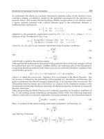
Abstract
In plasma physics, streamer pro pagation is an interesting discharge phenomenon
which has many applications in engineering and indust ry. Due to the small time
scale of streamer propagation, numerical simulation becomes a more effective way
to study the streamer than experiment. The governing partial different ial equa-
tions (PDEs) of streamer propagation include continuity equations for the particle

densities coupled with a Poisson’s equation for t he electric potential.
In this thesis, two discontinuo us Galerkin (DG) methods are proposed to solve
the continuity equations since there are large derivatives or even jumps in the pro-
file of particle densities. Meanwhile, the Poisson’s equation is solved by 4 differ-
ent methods which include finite difference method (FDM), mixed finite element
method (MFEM), least-squares finite element method (LSFEM), and symmetric in-
terior penalty Galerkin (SIPG) method. We have compared the compatibility when
these 4 methods are coupled with DG methods for cont inuity equations. The com-
parison results recommend that FDM is the b est method for Poisson’s equations if
uniform rectangular meshes are used and SIPG method is the b est choice for tri-
angular meshes. By applying the recommended methods, we have simulated many
configurations of short and long streamer propagations and successfully captured
the features of streamer.
vii
viii Abstract
In summary, this thesis work is a comprehensive study in applying DG meth-
ods to numerical simulations of streamer propagations. It supplements some early
numerical studies done by our collaborators. The gap lengths in most of the simula-
tions in our study are 5 times longer as the existing results, hence we have observed
more interesting phenomenon during simulations, for example the bifurcation of
streamer. We have considered not only the rectangular computatio na l domain in
this thesis, but also carried out simulat ion in complex geometry. Our study indicates
that DG method are highly potential competitor in simulating streamer propaga-
tions. In addition, this work studies the numerical compatibility in the coupling
between hyperbolic system and elliptic equation.
Key words: streamer propagations, hyperbolic system, coupling with ellip-
tic equation, discontinuous Galerkin methods, mixed finite element method, least-
squares finite element method.
Contents
Acknowledgements v

Abstract vii
List of Tables xv
List of Figures xix
1 Introduction 1
1.1 Background . . . . . . . . . . . . . . . . . . . . . . . . . . . . . . . . 1
1.2 Mathematical models . . . . . . . . . . . . . . . . . . . . . . . . . . . 3
1.2.1 Three-dimensional model . . . . . . . . . . . . . . . . . . . . . 5
1.2.2 Quasi three-dimensional mo del . . . . . . . . . . . . . . . . . 7
1.2.3 Two-dimensional model . . . . . . . . . . . . . . . . . . . . . 9
1.2.4 Quasi two-dimensional model . . . . . . . . . . . . . . . . . . 9
1.2.5 One-dimensional model . . . . . . . . . . . . . . . . . . . . . . 10
1.2.6 1.5-dimensional model . . . . . . . . . . . . . . . . . . . . . . 10
1.3 Literature Review . . . . . . . . . . . . . . . . . . . . . . . . . . . . . 1 2
ix
x Contents
1.4 Purpose . . . . . . . . . . . . . . . . . . . . . . . . . . . . . . . . . . 16
1.5 Outline . . . . . . . . . . . . . . . . . . . . . . . . . . . . . . . . . . . 17
2 Numerical Methods and Results for 1D Model 19
2.1 Numerical methods for Poisson’s equation . . . . . . . . . . . . . . . 20
2.1.1 The finite difference method . . . . . . . . . . . . . . . . . . . 20
2.1.2 The discontinuous Galerkin method . . . . . . . . . . . . . . . 21
2.1.3 The least-squares finite element method . . . . . . . . . . . . 23
2.2 Numerical methods for continuity equations . . . . . . . . . . . . . . 24
2.2.1 The Oden-Babuˇska-Baumann DG method . . . . . . . . . . . 25
2.2.2 The local discontinuous Galerkin method . . . . . . . . . . . . 26
2.2.3 Fully discrete formulation . . . . . . . . . . . . . . . . . . . . 28
2.2.4 The slope limiter . . . . . . . . . . . . . . . . . . . . . . . . . 29
2.3 Numerical comparisons and applicatio n . . . . . . . . . . . . . . . . . 30
2.4 A study of effects of para meters in source terms . . . . . . . . . . . . 34
3 Numerical Methods and Results for Quasi 2D Model 39

3.1 Numerical methods for Poisson’s equation . . . . . . . . . . . . . . . 41
3.1.1 The finite difference method . . . . . . . . . . . . . . . . . . . 41
3.1.2 The discontinuous Galerkin method . . . . . . . . . . . . . . . 42
3.1.3 The mixed finite element method . . . . . . . . . . . . . . . . 46
3.2 Numerical methods for continuity equations . . . . . . . . . . . . . . 49
3.2.1 The Oden-Babuˇska-Baumann DG method . . . . . . . . . . . 50
3.2.2 The local discontinuous Galerkin method . . . . . . . . . . . . 51
3.2.3 The slope limiter . . . . . . . . . . . . . . . . . . . . . . . . . 53
3.3 Numerical comparisons and applicatio ns . . . . . . . . . . . . . . . . 54
3.4 A study of effects of para meters in source terms . . . . . . . . . . . . 61
Contents xi
4 Numerical Methods and Results for 2D Model 65
4.1 Numerical methods for Poisson’s equation . . . . . . . . . . . . . . . 66
4.1.1 The finite difference method . . . . . . . . . . . . . . . . . . . 67
4.1.2 The discontinuous Galerkin method . . . . . . . . . . . . . . . 68
4.1.3 The mixed finite element method . . . . . . . . . . . . . . . . 70
4.1.4 The least-squares finite element method . . . . . . . . . . . . 72
4.2 Numerical method for continuity equatio ns . . . . . . . . . . . . . . . 73
4.2.1 The Oden-Babuˇska-Baumann DG method . . . . . . . . . . . 74
4.2.2 The slope limiter . . . . . . . . . . . . . . . . . . . . . . . . . 75
4.3 Numerical tests and comparisons . . . . . . . . . . . . . . . . . . . . 78
4.4 Numerical simulation . . . . . . . . . . . . . . . . . . . . . . . . . . . 81
5 Numerical Methods and Results for Quasi 3D Model 97
5.1 Numerical methods for Poisson’s equation . . . . . . . . . . . . . . . 98
5.1.1 The finite difference method . . . . . . . . . . . . . . . . . . . 99
5.1.2 The discontinuous Galerkin methods . . . . . . . . . . . . . . 100
5.1.3 The mixed finite element method . . . . . . . . . . . . . . . . 104
5.1.4 The least-squares finite element method . . . . . . . . . . . . 105
5.2 Numerical method for continuity equatio ns . . . . . . . . . . . . . . . 106
5.2.1 The Oden-Babuˇska-Baumann DG method . . . . . . . . . . . 106

5.2.2 The slope limiter . . . . . . . . . . . . . . . . . . . . . . . . . 107
5.3 Numerical tests and comparisons . . . . . . . . . . . . . . . . . . . . 108
5.4 Numerical simulation . . . . . . . . . . . . . . . . . . . . . . . . . . . 113
5.5 Quasi 3D model v.s. 1.5 D model . . . . . . . . . . . . . . . . . . . . 120
6 Conclusions 135
Bibliography 150

List of Tables
2.1 Number of unknowns in one single time step for different methods in
1D comparison. . . . . . . . . . . . . . . . . . . . . . . . . . . . . . . 31
2.2 Error and convergence rate for σ in 1D comparison. . . . . . . . . . . 32
2.3 Error and convergence rate for ρ in 1D comparison. . . . . . . . . . . 32
2.4 Error and convergence rate for φ in 1D comparison. . . . . . . . . . . 33
2.5 Error and convergence rate for E in 1D comparison. . . . . . . . . . . 33
3.1 Error and convergence rate for φ in Example 1 of quasi 2D test. . . . 48
3.2 Error and convergence rate for E = −φ
′
in Example 1 of quasi 2 D test. 48
3.3 Error and convergence rate for φ in Example 2 of quasi 2D test. . . . 49
3.4 Error and convergence rate for E = −φ
′
in Example 2 of quasi 2 D test. 50
3.5 Error and convergence rate for σ in Accuracy test 1 of quasi 2D
comparison. . . . . . . . . . . . . . . . . . . . . . . . . . . . . . . . . 55
3.6 Error and convergence rat e for ρ in Accuracy test 1 of quasi 2D com-
parison. . . . . . . . . . . . . . . . . . . . . . . . . . . . . . . . . . . 56
3.7 Error and convergence rate for φ in Accuracy test 1 of quasi 2D
comparison. . . . . . . . . . . . . . . . . . . . . . . . . . . . . . . . . 56
xiii
xiv List of Tables

3.8 Error and convergence rate for E in Accuracy test 1 of quasi 2D
comparison. . . . . . . . . . . . . . . . . . . . . . . . . . . . . . . . . 57
3.9 Error and convergence rate for σ in Accuracy test 2 of quasi 2D
comparison. . . . . . . . . . . . . . . . . . . . . . . . . . . . . . . . . 58
3.10 Error and convergence rate for ρ in Accuracy test 2 of quasi 2D com-
parison. . . . . . . . . . . . . . . . . . . . . . . . . . . . . . . . . . . 59
3.11 Error and convergence ra t e for φ in Accuracy test 2 of quasi 2D
comparison. . . . . . . . . . . . . . . . . . . . . . . . . . . . . . . . . 59
3.12 Error and convergence rate for E in Accuracy test 2 of quasi 2D
comparison. . . . . . . . . . . . . . . . . . . . . . . . . . . . . . . . . 60
4.1 Complexity for different methods to solve Poisson’s equation in 2D
model. . . . . . . . . . . . . . . . . . . . . . . . . . . . . . . . . . . . 78
4.2 Error and convergence rate fo r σ in 2D co mpar ison based on rectan-
gular mesh. . . . . . . . . . . . . . . . . . . . . . . . . . . . . . . . . 79
4.3 Error and convergence rate for ρ in 2D comparison based on rectan-
gular mesh. . . . . . . . . . . . . . . . . . . . . . . . . . . . . . . . . 80
4.4 Error and convergence rate for φ in 2D comparison based on rectan-
gular mesh. . . . . . . . . . . . . . . . . . . . . . . . . . . . . . . . . 80
4.5 Error and convergence rate for σ in 2D comparison based on triangu-
lar mesh. . . . . . . . . . . . . . . . . . . . . . . . . . . . . . . . . . . 82
4.6 Error and convergence rate for ρ in 2D comparison based on tria ngular
mesh. . . . . . . . . . . . . . . . . . . . . . . . . . . . . . . . . . . . . 8 2
4.7 Error and convergence rate for φ in 2D compar ison based on triangu-
lar mesh. . . . . . . . . . . . . . . . . . . . . . . . . . . . . . . . . . . 83
4.8 Error and convergence rate for E in 2D comparison ba sed on trian-
gular mesh. . . . . . . . . . . . . . . . . . . . . . . . . . . . . . . . . 83
List of Tables xv
4.9 Memory cost for different methods in 2D comparison based on trian-
gular mesh. . . . . . . . . . . . . . . . . . . . . . . . . . . . . . . . . 84
5.1 Error and convergence rate for σ in quasi 3D comparison based on

rectangular mesh. . . . . . . . . . . . . . . . . . . . . . . . . . . . . . 108
5.2 Error and convergence rate for ρ in quasi 3D comparison based on
rectangular mesh. . . . . . . . . . . . . . . . . . . . . . . . . . . . . . 109
5.3 Error and convergence rate for φ in quasi 3D comparison based on
rectangular mesh. . . . . . . . . . . . . . . . . . . . . . . . . . . . . . 109
5.4 Error and convergence rate for φ in quasi 3D comparison based on
triangular mesh. . . . . . . . . . . . . . . . . . . . . . . . . . . . . . . 111
5.5 Error and convergence rate for −
∂φ
∂r
in quasi 3D comparison based on
triangular mesh. . . . . . . . . . . . . . . . . . . . . . . . . . . . . . . 111
5.6 Error and convergence rate for −
∂φ
∂z
in quasi 3D comparison based on
triangular mesh. . . . . . . . . . . . . . . . . . . . . . . . . . . . . . . 112
5.7 Error and convergence rate for SIPG+OBBDG method in quasi 3D
test on triangular mesh. . . . . . . . . . . . . . . . . . . . . . . . . . 112

List of Figures
1.1 A schematic representation of streamer . . . . . . . . . . . . . . . . . 4
1.2 The computational domain o f quasi 3D model. . . . . . . . . . . . . . 8
2.1 Double headed streamer propagation in 1D simulation. . . . . . . . . 35
2.2 Effects of different K on particle densities in 1D simulation. . . . . . 36
2.3 Effects of different S on particle densities in 1D simulation. . . . . . . 37
2.4 Effects of different S and K on electric potential and field in 1D
simulation. . . . . . . . . . . . . . . . . . . . . . . . . . . . . . . . . . 38
3.1 The dynamics results of a quasi 2D simulation. . . . . . . . . . . . . . 60
3.2 Effects of different S or K on maximum particle densities in quasi 2D

simulation. . . . . . . . . . . . . . . . . . . . . . . . . . . . . . . . . . 62
3.3 Effects of different S or K on net charge density in quasi 2D simulation. 63
3.4 Effects of different S or K on the electric potential and field in quasi
2D simulation. . . . . . . . . . . . . . . . . . . . . . . . . . . . . . . . 64
4.1 Boundary conditions for 2D model. . . . . . . . . . . . . . . . . . . . 66
xvii
xviii List of Figures
4.2 The avera ge time cost in one single step for each method in the nu-
merical tests under tr iangular mesh. . . . . . . . . . . . . . . . . . . . 84
4.3 The distribution of electron density (m
−3
) at 10ns (left) and 15ns
(right). . . . . . . . . . . . . . . . . . . . . . . . . . . . . . . . . . . . 88
4.4 The distribution of electron density (m
−3
) at 20ns. . . . . . . . . . . 89
4.5 The distribution of electron density (m
−3
) at 25ns (left) and 30ns
(right). . . . . . . . . . . . . . . . . . . . . . . . . . . . . . . . . . . . 90
4.6 The distribution of electron density (m
−3
) at 35ns (left) and 40ns
(right). . . . . . . . . . . . . . . . . . . . . . . . . . . . . . . . . . . . 91
4.7 The distribution of net charge density (m
−3
, left) and electric field
|E| (kV/m, right) at 10ns. . . . . . . . . . . . . . . . . . . . . . . . . 9 2
4.8 The distribution of net charge density (m
−3

, left) and electric field
|E| (kV/m, right) at 30ns. . . . . . . . . . . . . . . . . . . . . . . . . 9 3
4.9 The distribution of net charge density (m
−3
, left) and electric field
|E| (kV/m, right) at 35ns. . . . . . . . . . . . . . . . . . . . . . . . . 9 4
4.10 The distribution of net charge density (m
−3
) at 25, 30, 35 and 40ns
(from left to right). . . . . . . . . . . . . . . . . . . . . . . . . . . . . 9 5
4.11 The distribution of electric field |E| (V /m) at 25, 30, 35 and 4 0ns
(from left to right). . . . . . . . . . . . . . . . . . . . . . . . . . . . . 9 6
5.1 Boundary conditions for quasi 3D model. . . . . . . . . . . . . . . . . 98
5.2 The z-component of electric field (V/cm) along z-axis a t 1ns and 2ns
in the simulation for nitrogen. . . . . . . . . . . . . . . . . . . . . . . 115
5.3 The evolution of z-component of electric field ( V /cm) along z-axis
from 2ns to 5ns in the simulation for nitrogen. . . . . . . . . . . . . . 116
5.4 The evolution of average speed (cm/s, top) and maximum density
(cm
−3
, bottom) of positive and negative str eamer along z-axis in the
simulation for nitrogen. . . . . . . . . . . . . . . . . . . . . . . . . . . 122
List of Figures xix
5.5 The distribution of electric field |E| ( V /cm) and net charge density
(cm
−3
) at 2ns in the simula t ion wit hin nitrogen. . . . . . . . . . . . . 123
5.6 The distribution of electric field |E| ( V /cm) and net charge density
(cm
−3

) at 4ns in the simula t ion wit hin nitrogen. . . . . . . . . . . . . 124
5.7 The distribution of different particles along axial direction at 1ns in
the simulation in SF
6
. . . . . . . . . . . . . . . . . . . . . . . . . . . 125
5.8 The evolution of z-component of electric field alo ng axial direction in
the simulation in SF
6
. . . . . . . . . . . . . . . . . . . . . . . . . . . 126
5.9 The distribution of net charge density (µC/cm
3
) at 1ns in the simu-
lation in SF
6
. . . . . . . . . . . . . . . . . . . . . . . . . . . . . . . . 127
5.10 The distribution of electric field |E| (kV/cm) at 1ns in the simulation
in SF
6
. . . . . . . . . . . . . . . . . . . . . . . . . . . . . . . . . . . . 128
5.11 The evolution of electron density (cm
−3
, top) and z-component o f
electric field (kV/cm, bottom) along the z-axis in point -to-plane stream-
er propagation simulat ion. . . . . . . . . . . . . . . . . . . . . . . . . 129
5.12 The evolution of net particle density (cm
−3
) in point-to-plane stream-
er propagation simulat ion. . . . . . . . . . . . . . . . . . . . . . . . . 130
5.13 The evolution of electric field |E| (kV/cm) in point-to-plane streamer
propagation simulation. . . . . . . . . . . . . . . . . . . . . . . . . . . 131

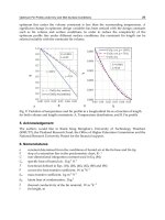
5.14 The electric field (kV /cm) along axial direction under different values
of r
d
. The benchmark is given by quasi 3D simulation. . . . . . . . . 132
5.15 The electric field (kV /cm) along axial direction under different values
of r
d
. This figure is used to show the limiting solution when r
d
→ ∞. 133

Chapter 1
Introduction
1.1 Background
In physics, plasma is a state of matter in which a certain port ion of the particles are
ionized [56]. When non-ionized o r lowly ionized matter is exposed to high electric
field, non-equilibrium ionization processes, so-called discharges, occur. In recent
years, plasma discharges have been studied in industrial and technical applications
[17, 74, 91]. A particular example of plasma discharges is lightning, which is still a
big problem and needs to be aboratively studied. Another interesting experiment al
example is the breakdown in air ga p which is submitted to a very high, in magnitude,
voltage at atmospheric pressure [47, 65 ].
Consider two metal electrodes, anode and cathode, which are separated by a
gas-filled gap. Up to a certain threshold value of applied electric field, free electrons
are produced by ionizations. When the free electron forms an electron avalanche,
the so-called first coro na inception occurs [34]. In a positive discharge where the gap
is submitted to a po sitive voltage, the electron avalanche moving towards the anode
creates a net positive charge which increases the electric field near the avalanche.
If the modified electric field is high enough, new avalanches can be generated and
developed. The discharge process then consists of a series of avalanches developing

1
2 Chapter 1. Introduction
into narrow branched plasma channels, which are called streamers. These channels
develop from a common root. On the other hand, if a negative voltag e is applied to
the air gap, the first corona will disappear after some time; and then two coronas of
opposite polarity, positive corona and negative corona, develop after the extinction
of the first corona.
If the gap is long enough such that breakdown occurs after a large time scale,
a new phenomenon called leader will be observed. In positive discharge, leader
appears as a weakly luminous channel from the common root of positive streamer,
and then elongates and propagates cont inuously, and also pushes the streamer. On
the other hand, in negative discharge, since positive corona propagates towards
the H.V. electrode and negative coro na moves in the opposite way, a new leader
channel occurs between them. This leader is called space leader and elongates bi-
directionally. Therefore, a j unction of space leader and original leader will produce
a strong illumination of the whole channel.
The mechanism of streamer and leader has been studied in the past three decades
[49, 51, 59, 68, 72, 79]. Firstly, the minimum inception field of the first corona is
empirically given by the Peek’s equation [75]
E = E
0
δM

1 +
K
√
δR

,
where E

0
is the breakdown field in the range of 10
6
V/m, δ is relative air density, R is
equivalent curvature radius of electrode, K and M a re two constants. This formula
is just one of the various criteria [1, 45, 55, 66, 67] fo r the inception of streamer. This
inception process can continue for several microseconds during the propagation of
streamers as long as the electric field around the tip of streamers is sufficiently large.
The streamer usually propagat es with velocity in the range of 10
7
cm/s; therefore, in
the short gap (in the millimeter or centimeter range), breakdown occurs in several
nanoseconds.
On the other ha nd, in the elongation of leader, since the electrons and positive
ions travel in opposite direction in the leader channel, current is created. Then the
1.2 Mathematical models 3
thermal energy in the leader channel will be increased by the current due to Joule
effect. Thus, different from the mechanism of streamer, leader is governed by a
thermal process. The diameter of leader channel is propor tional to the length of
the gap. It is between 0.5 and 1mm for a 1.5m gap and between 2 and 4mm for a
10m gap. The temperat ur e in leader channel can reach several thousands of Kelvin.
This elongation process can continue for several hundred microseconds.
For a better understanding of streamer a nd leader, one can refer to the schematic
representation in Figure 1.1, which is cited from [33],
So far, the most common method fo r studying streamer discharges is still to
do the experiments [16, 34, 39, 80, 81, 82, 83, 90]. However, the above small time
scales of the discharge processes regretfully indicate tha t it is difficult to acquire
exp erimental data. Therefore, more researchers start to develop proper physical
and mathematical models and do accurate numerical simulations to study streamer
propagation.

1.2 Mathematical models
Based on experimental studies, scientists have developed many different empirical
models, for example the Critical Volume Model proposed by the Renardi`eres Group
[81] and its modifications [4 , 27, 77], some models for describing the branching
phenomenon of streamer [2, 69] and static models for space charges [23, 42, 94].
These empirical models are ba sed on some empirical formulas; as a result, they
usually amplify some features during the streamer propagation process but neglect
some other features. For example in [2], the authors took too much care about
the randomness of streamer propagation; hence their st r eamer channels spread out
around the tip electrode and seldom propagated to the other electrode. Thus, some
kinetic models are developed to overcome this problem. For instant, the kinetic
model with Monte Carlo simulat ion [48] and particle-in-cell (PIC) model [78, 87]
use the so-called superparticle (clouds of particles) instead of as single particle.
4 Chapter 1. Introduction
Figure 1.1: This figure shows the well-developed streamer and leader. The ”corona
glow” is also called streamer.
Although kinetic models can simulate the streamer propagation mo r e exactly, it
is still difficult to implement because of the la rge computational co st. Therefore,
fluid models have been widely accepted and provided good descriptions of discharge
processes [38, 76, 93, 97].
1.2 Mathematical models 5
1.2.1 Three-dimensional model
The most common fluid model for streamer propagation is a three-dimensional (3D)
model which contains three continuity equations for particle densities of electron N
e
,
positive ion N
p
and negative ion N
n

, and a Poisson’s equation for electric potential
V as follows,



















∂N
e
∂t
+ ∇· (N
e
W
e
− D∇N
e

) = (α(|E|) − η(|E|))N
e
|W
e
| −βN
e
N
p
+ S
ph
(N
e
, E),
∂N
p
∂t
+ ∇· (N
p
W
p
) = α( |E|)N
e
|W
e
| −βN
e
N
p
− βN
n

N
p
+ S
ph
(N
e
, E),
∂N
n
∂t
+ ∇· (N
n
W
n
) = η(|E|)N
e
|W
e
| −βN
n
N
p
,
−∇
2
V =
e
ǫ
(N
p

− N
e
− N
n
), E = −∇V.
(1.1)
In (1.1), W
e
, W
p
and W
n
are the drift velocities for electron, positive ion and
negative ion respectively, which equal to the electric field E multiplied by mobility
µ
e
, µ
p
and µ
n
, i.e. W
e,p,n
= µ
e,p,n
E; D is the diffusion tensor; α(|E|) is an impact
ionization coefficient described with Townsend’s approximation [80], i.e., α(|E|) =
AP e
BP/|E|
, where P is the air pressure in torr and A, B are two parameters. η(|E|) is
the electron attachment coefficient and β is the recombination coefficient. S

ph
(N
e
, E)
is the photoionization source which can be calculated either by the integral method
of Zheleznyak et al. [100] or by solving a set of Helmholtz equa tions [13, 57, 73];
this source term can be neglected in negative streamer [62] or can be equivalent
to the background ionization under certain conditions [7, 96]. The constants e
and ǫ are called elementary charge and permittivity of vacuum respectively. The
physical domain in model (1.1) is the whole space between anode and cathode,
therefore we impose the Dirichlet boundary conditions for Poisson’s equation at the
electrodes. We allow the flux of particles to pass through the boundaries [62], thus
we impose homogeneous Neumann boundary conditions for continuity equations at
the electrodes.
Various modificatio ns of (1.1) exist in the literature. For example, C. Montijn