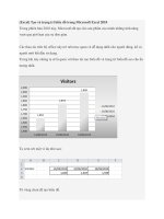
Microsoft excel 2010 advanced

Stephen Mofat, The Mouse Training Company

Excel 2010 Advanced

Download free ebooks at bookboon.com

2


Excel 2010 Advanced

Excel 2010 Advanced
© 2011 Stephen Mofat, The Mouse Training Company & Ventus Publishing ApS
ISBN 978-87-7681-788-6

Download free ebooks at bookboon.com

3


Excel 2010 Advanced

Contents

Contents
1

2

3

Introduction

7

Advanced worksheet functions

9

Conditional & Logical Functions

10

Counting And Totalling Cells Conditionally

14

And, Or, Not

25

Lookup Functions

31

Views, scenarios, goal seek, solver

39

Goal Seeking And Solving

40

Advanced Solver Features

47

Scenarios

51

Views

59

Using excel to manage lists

64

Excel Lists,List Terminology

64

Sorting Data

65

Subtotals

73

Filtering A List

79

Advanced Filtering

87

Please click the advert

Fast-track
your career
Masters in Management

Stand out from the crowd
Designed for graduates with less than one year of full-time postgraduate work
experience, London Business School’s Masters in Management will expand your
thinking and provide you with the foundations for a successful career in business.
The programme is developed in consultation with recruiters to provide you with
the key skills that top employers demand. Through 11 months of full-time study,
you will gain the business knowledge and capabilities to increase your career
choices and stand out from the crowd.

London Business School
Regent’s Park
London NW1 4SA
United Kingdom
Tel +44 (0)20 7000 7573
Email

Applications are now open for entry in September 2011.

For more information visit www.london.edu/mim/
email or call +44 (0)20 7000 7573

www.london.edu/mim/

Download free ebooks at bookboon.com

4


4

Please click the advert

5

Contents

Criteria Tips

91

Multiple Criteria

93

Calculated Criteria

94

Data Consolidation

102

Pivottables

106

Modifying A Pivottable

117

Managing Pivottables

123

Formatting A Pivottable

130

Banding

131

Slicers

135

Charts

143

Introduction To Charting

143

Creating Charts

145

Formatting Charts

157

Changing he Chart Layout

163

Sparklines

177

Templates

184

Introduction To Templates

185

Create Custom Templates

187

You’re full of energy
and ideas. And that’s
just what we are looking for.

© UBS 2010. All rights reserved.

Excel 2010 Advanced

Looking for a career where your ideas could really make a difference? UBS’s
Graduate Programme and internships are a chance for you to experience
for yourself what it’s like to be part of a global team that rewards your input
and believes in succeeding together.
Wherever you are in your academic career, make your future a part of ours
by visiting www.ubs.com/graduates.

www.ubs.com/graduates

Download free ebooks at bookboon.com

5


Excel 2010 Advanced

6

Drawing and formatting

194

Inserting, Formatting And Deleting Objects

195

More Formatting

209

Excel tools

227

Reviewing

228

Auditing

245

Prooing Tools

251

Please click the advert

7

Contents

Download free ebooks at bookboon.com

6


Excel 2010 Advanced

Introduction

Introduction
Excel 2010 is a powerful spreadsheet application that allows users to produce tables containing calculations and graphs.
hese can range from simple formulae through to complex functions and mathematical models.

How To Use This Guide
his manual should be used as a point of reference ater following attendance of the advanced level Excel 2010 training
course. It covers all the topics taught and aims to act as a support aid for any tasks carried out by the user ater the course.
he manual is divided into sections, each section covering an aspect of the advanced course. he table of contents lists
the page numbers of each section and the table of igures indicates the pages containing tables and diagrams.

Objectives
Sections begin with a list of objectives each with its own check box so that you can mark of those topics that you are
familiar with following the training.

Instructions
hose who have already used a spreadsheet before may not need to read explanations on what each command does, but
would rather skip straight to the instructions to ind out how to do it. Look out for the arrow icon which precedes a list
of instructions.

Appendices
he Appendices list the Ribbons mentioned within the manual with a breakdown of their functions and tables of shortcut
keys.
Keyboard
Keys are referred to throughout the manual in the following way:
[ENTER] – Denotes the return or enter key, [DELETE] – denotes the Delete key and so on.
Where a command requires two keys to be pressed, the manual displays this as follows:
[CTRL] + [P] – this means press the letter “p” while holding down the Control key.
Commands
When a command is referred to in the manual, the following distinctions have been made:

Download free ebooks at bookboon.com

7


Excel 2010 Advanced

Introduction

When Ribbon commands are referred to, the manual will refer you to the Ribbon – E.g. “Choose home from the Ribbons
the group name – FONT group and then B for bold”.
When dialog box options are referred to, the following style has been used for the text – “In the PAGE RANGE section
of the PRINT dialog, click the CURRENT PAGE option”
Dialog box buttons are shaded and boxed – “Click OK to close the PRINT dialog and launch the print.”

Notes
Within each section, any items that need further explanation or extra attention devoted to them are denoted by shading.
For example:
“Excel will not let you close a ile that you have not already saved changes to without prompting you to save.”
Tips
At the end of each section there is a page for you to make notes on and a “Useful Information” heading where you will
ind tips and tricks relating to the topics described within the section.

Download free ebooks at bookboon.com

8


Excel 2010 Advanced

Advanced worksheet functions

1 Advanced worksheet functions
By the end of this section you will be able to:
• Understand and use conditional formulae
• Set up LOOKUP tables and use LOOKUP functions
• Use the GOAL SEEK
• Use the SOLVER

Download free ebooks at bookboon.com

9


Excel 2010 Advanced

Advanced worksheet functions

Conditional & Logical Functions
Excel has a number of logical functions which allow you to set various “conditions” and have data respond to them. For
example, you may only want a certain calculation performed or piece of text displayed if certain conditions are met. he
functions used to produce this type of analysis are found in the Insert, Function menu, under the heading LOGICAL.

If Statements
he IF function is used to analyse data, test whether or not it meets certain conditions and then act upon its decision. he
formula can be entered either by typing it or by using the Function Library on the formula’s ribbon, the section that deals
with logical functions Typically, the IF statement is accompanied by three arguments enclosed in one set of parentheses;
the condition to be met (logical_test); the action to be performed if that condition is true (value_if_true); the action to
be performed if false (value_if_false). Each of these is separated by a comma, as shown;
=IF ( logical_test, value_if_true, value_if_false)
To view IF function syntax:
Mouse
1. Click the drop down arrow next to the LOGICAL button in the FUNCTION LIBARY Groupon the
FORMULAS Ribbon;
2. A dialog box will appear
3. he three arguments can be seen within the box

Download free ebooks at bookboon.com

10


Excel 2010 Advanced

Advanced worksheet functions

Logical Test
his part of the IF statement is the “condition”, or test. You may want to test to see if a cell is a certain value, or to compare
two cells. In these cases, symbols called LOGICAL OPERATORS are useful;
>

Greater than

<

Less than

>=

Greater than or equal to

<=

Less than or equal to

=

Equal to

<>

Not equal to

Therefore, a typical logical test might be B1>B2, testing whether or not the value contained in cell B1 of the
spreadsheet is greater than the value in cell B2. Names can also be included in the logical test, so if cells B1 and B2 were

respectively named SALES and TARGET, the logical test would read SALES>TARGET. Another type of logical test could
include text strings. If you want to check a cell to see if it contains text, that text string must be included in quotation
marks. For example, cell C5 could be tested for the word YES as follows; C5=”YES”.
It should be noted that Excel’s logic is, at times, brutally precise. In the above example, the logical test is that sales should
be greater than target. If sales are equal to target, the IF statement will return the false value. To make the logical test
more lexible, it would be advisable to use the operator >= to indicate “meeting or exceeding”.

Value If True / False
Provided that you remember that TRUE value always precedes FALSE value, these two values can be almost anything.
If desired, a simple number could be returned, a calculation performed, or even a piece of text entered. Also, the type
of data entered can vary depending on whether it is a true or false result. You may want a calculation if the logical test
is true, but a message displayed if false. (Remember that text to be included in functions should be enclosed in quotes).

Download free ebooks at bookboon.com

11


Excel 2010 Advanced

Advanced worksheet functions

Taking the same logical test mentioned above, if the sales igure meets or exceeds the target, a BONUS is calculated (e.g.
2% of sales). If not, no bonus is calculated so a value of zero is returned. he IF statement in column D of the example
reads as follows;
=IF(B2>=C2,B2*2%,0)

You may, alternatively, want to see a message saying “NO BONUS”. In this case, the true value will remain the same and
the false value will be the text string “NO BONUS”;
=IF(B2>=C2,B2*2%,”NO BONUS”)

your chance
Please click the advert

to change

the world
Here at Ericsson we have a deep rooted belief that
the innovations we make on a daily basis can have a
profound effect on making the world a better place
for people, business and society. Join us.
In Germany we are especially looking for graduates
as Integration Engineers for
• Radio Access and IP Networks
• IMS and IPTV
We are looking forward to getting your application!
To apply and for all current job openings please visit
our web page: www.ericsson.com/careers

Download free ebooks at bookboon.com

12


Excel 2010 Advanced

Advanced worksheet functions

A particularly common use of IF statements is to produce “ratings” or “comments” on igures in a spreadsheet. For this,
both the true and false values are text strings. For example, if a sales igure exceeds a certain amount, a rating of “GOOD”

is returned, otherwise the rating is “POOR”;
=IF(B2>1000,”GOOD”,”POOR”)

Nested If
When you need to have more than one condition and more than two possible outcomes, a NESTED IF is required. his
is based on the same principle as a normal IF statement, but involves “nesting” a secondary formula inside the main one.
he secondary IF forms the FALSE part of the main statement, as follows;
=IF(1st logic test , 1st true value , IF(2nd logic test , 2nd true value , false value))
Only if both logic tests are found to be false will the false value be returned. Notice that there are two sets of parentheses,
as there are two separate IF statements. his process can be enlarged to include more conditions and more eventualities up to seven IF’s can be nested within the main statement. However, care must be taken to ensure that the correct number
of parentheses are added.
In the example, sales staf could now receive one of three possible ratings;
=IF(B2>1000,”GOOD”,IF(B2<600,”POOR”,”AVERAGE”))
To make the above IF statement more lexible, the logical tests could be amended to measure sales against cell references
instead of igures. In the example, column E has been used to hold the upper and lower sales thresholds.
=IF(B2>$E$2,”GOOD”,IF(B2<$E$3,”POOR”,”AVERAGE”))
(If the IF statement is to be copied later, this cell reference should be absolute).

N.B. he depth of nested IF functions has been increased to 64 as previous versions of excel only nested 7 deep

Download free ebooks at bookboon.com

13


Excel 2010 Advanced

Advanced worksheet functions

Counting And Totalling Cells Conditionally

Occasionally you may need to create a total that only includes certain cells, or count only certain cells in a column or row.

he example above shows a list of orders. here are two headings in bold at the bottom where you need to generate a) the
total amount of money spent by Viking Supplies and b) the total number of orders placed by Bloggs & Co.
he only way you could do this is by using functions that have conditions built into them. A condition is simply a test
that you can ask Excel to carry out the result of which will determine the result of the function.

Statistical If Statements
A very useful technique is to display text or perform calculations only if a cell is the maximum or minimum of a range. In
this case the logical test will contain a nested statistical function (such as MAX or MIN). If, for example, a person’s sales
cell is the maximum in the sales column, a message stating “Top Performer” could appear next to his or her name. If the
logical test is false, a blank message could appear by simply including an empty set of quotation marks. When typing the
logical test, it should be understood that there are two types of cell referencing going on. he irst is a reference to one
person’s igure, and is therefore relative. he second reference represents the RANGE of everyone’s igures, and should
therefore be absolute.
=IF(relative cell = MAX(absolute range) , “Top Performer” , “”)

Download free ebooks at bookboon.com

14


Excel 2010 Advanced

Advanced worksheet functions

In this example the IF statement for cell B2 will read;
=IF(C2=MAX($C$2:$C$4),”Top Performer”,””)
When this is illed down through cells B3 and B4, the irst reference to the individual’s sales igure changes, but the
reference to all three sales igures ($C$2:$C$4) should remain constant. By doing this, you ensure that the IF statement

is always checking to see if the individual’s igure is the biggest out of the three.
A further possibility is to nest another IF statement to display a message if a value is the minimum of a range. Beware of
syntax here - the formula could become quite unwieldy!
e Graduate Programme
for Engineers and Geoscientists

I joined MITAS because
I wanted real responsibili

Please click the advert

Maersk.com/Mitas

Real work
Internationa
al opportunities
International
ree work
wo
or placements

Month 16
I was a construction
supervisor in
the North Sea
advising and
he
helping foremen
ssolve problems
Download free ebooks at bookboon.com

15


Excel 2010 Advanced

Advanced worksheet functions

Sumif
You can use this function to say to Excel, “Only total the numbers in the Total column where the entry in the Customer
column is Viking Supplies”. he syntax of the SUMIF() function is detailed below:
=SUMIF(range,criteria,sum_range)
RANGE is the range of cells you want to test.
CRITERIA. It is the criteria in the form of a number, expression, or text that deines which cells will be added. For
example, criteria can be expressed as 32, “32”, “>32”, “apples”.
SUM RANGE. hese are the actual cells to sum. he cells in sum range are summed only if their corresponding cells in
range match the criteria. If sum range is omitted, the cells in range are summed.

=SUMIF(B2:B11, “Viking Supplies”, F2:F11)
With the example above, the SUMIF function that you would use to generate the VIKING SUPPLIES TOTAL would
look as above.
Using the INSERT FUNCTION tool the dialog would look like this and show any errors in entering the values or ranges

Download free ebooks at bookboon.com

16


Excel 2010 Advanced

Advanced worksheet functions

Countif
countif counts the number of cells in a range based on agiven criteria.
COUNTIF(range,criteria)
RANGEis one or more cells to count, including numbers or names, arrays, or references that contain numbers. Blank
and text values are ignored.
CRITERIAIS the criteria in the form of a number, expression, cell reference, or text that deines which cells will be
counted. For example, criteria can be expressed as 32, “32”, “>32”, “apples”, or B4.
To use COUNTIF function
Mouse
1. Click on the MORE FUNCTIONS button in the FORMULAS group on the FORMULAS ribbon
2. Click on STATISTICAL.
3. Select COUNTIF from the displayed functions. A dialog will be displayed

Download free ebooks at bookboon.com

17


Excel 2010 Advanced

Advanced worksheet functions

4. Click in RANGE text box
5. Select the range of cells you wish to check.
6. Click in the CRITERIA box, either, type criteria directly in the box or select a cell that contains the value
you wish to count.
7. Click OK

Averageif
A very common request is for a single function to conditionally average a range of numbers – a complement to SUMIF
and COUNTIF. AVERAGEIF, allows users to easily average a range based on a speciic criteria.

Brain power
Please click the advert

By 2020, wind could provide one-tenth of our planet’s
electricity needs. Already today, SKF’s innovative knowhow is crucial to running a large proportion of the
world’s wind turbines.
Up to 25 % of the generating costs relate to maintenance. These can be reduced dramatically thanks to our
systems for on-line condition monitoring and automatic
lubrication. We help make it more economical to create
cleaner, cheaper energy out of thin air.
By sharing our experience, expertise, and creativity,
industries can boost performance beyond expectations.
Therefore we need the best employees who can
meet this challenge!

The Power of Knowledge Engineering

Plug into The Power of Knowledge Engineering.
Visit us at www.skf.com/knowledge

Download free ebooks at bookboon.com

18


Excel 2010 Advanced

Advanced worksheet functions

AVERAGEIF(Range, Criteria, [Average Range])
RANGEis one or more cells to average, including numbers or names, arrays, or references that contain numbers.
CRITERIAIS the criteria in the form of a number, expression, cell reference, or text that deines which cells are averaged.
For example, criteria can be expressed as 32, “32”, “>32”, “apples”, or B4.
AVERAGe_rangeis the actual set of cells to average. If omitted, RANGE is used.
Here is an example that returns the average of B2:B5 where the corresponding value in column A is greater than 250,000:
=AVERAGEIF(A2:A5, “>250000”, B2:B5)
To use AVERAGEIF function
Mouse
1. Click on the MORE FUNCTIONS button in the FORMULAS group on the FORMULAS ribbon and Click
on STATISTICAL.
2. SelectAVERAGEIF from the displayed functions. A dialog will be displayed

3. Click in RANGE text box.
4. Select the range of cells containing the .values you wish checked against the criteria.
5. Click in the CRITERIA box, either, type criteria directly in the box or select a cell that contains the value
you wish to check the range against.
6. Click in the AVERAGE_RANGE text box and select the range you wish to average..
7. Click ok.

Averageifs
Average ifs is a new function to excel and does much the same as the Averageif function but it will average a range using
multiple criteria.
Download free ebooks at bookboon.com

19

Excel 2010 Advanced

Advanced worksheet functions

To use AVERAGEIFS function
Mouse
1. Click on the MORE FUNCTIONS button in the FORMULAS group on the FORMULAS ribbon and Click
on STATISTICAL.
2. SelectAVERAGEIFS from the displayed functions. A dialog will be displayed.

3. Click in AVERAGE_RANGE text box.
4. Select the range of cells containing the .values you wish checked against the criteria.
5. Click in the CRITERIA_RANGE1 box select a range of cells that contains the values you wish to check the
criteria against.
6. Click in the CRITERIA1Text box and type in the criteria to measure against your CRITERIA_RANGE1.
7. Repeat steps 5 and 6 to enter multiple criteria, range2, range3 etc, use the scroll bar on the right to scroll
down and locate more range and criteria text boxes.Click OK when all ranges and criterias have been
entered.
Some important points about AVERAGEIFS function
Download free ebooks at bookboon.com

20


Excel 2010 Advanced

Advanced worksheet functions

• If AVERAGE_RANGE is a blank or text value, AVERAGEIFS returns the #DIV0! error value.

• If a cell in a criteria range is empty, AVERAGEIFS treats it as a 0 value.
• Cells in range that contain TRUE evaluate as 1; cells in range that contain FALSE evaluate as 0 (zero).
• Each cell in average_range is used in the average calculation only if all of the corresponding criteria speciied
are true for that cell.
• Unlike the range and criteria arguments in the AVERAGEIF function, in AVERAGEIFS each CRITERIA_
RANGE must be the same size and shape as sum_range.
• If cells in AVERAGE_RANGE cannot be translated into numbers, AVERAGEIFSreturns the #DIV0! error
value.
• If there are no cells that meet all the criteria, AVERAGEIFSreturns the #DIV/0! error value.
• You can use the wildcard characters, question mark (?) and asterisk (*), in criteria. A question mark matches
any single character; an asterisk matches any sequence of characters. If you want to ind an actual question
mark or asterisk, type a tilde (~) before the character.

Please click the advert

Are you considering a
European business degree?

LEARN BUSINESS at university
level.
We mix cases with cutting edg
e
research working individual
ly or in
teams and everyone speaks
English.
Bring back valuable knowle
dge and
experience to boost your car
eer.

MEET a culture of new foods,
music
and traditions and a new way
of
studying business in a safe,
clean
environment – in the middle
of
Copenhagen, Denmark.

ENGAGE in extra-curricular act
ivities
such as case competitions,
sports,
etc. – make new friends am
ong cbs’
18,000 students from more
than 80
countries.

See what we look like
and how we work on cbs.dk

Download free ebooks at bookboon.com

21


Excel 2010 Advanced

Advanced worksheet functions

Sumifs
his function adds all the cells in a range that meets multiple criteria.
he order of arguments is diferent between SUMIFS and SUMIF. In particular, the SUM_RANGE argument is the irst
argument in SUMIFS, but it is the third argument in SUMIF. If you are copying and editing these similar functions, make
sure you put the arguments in the correct order.
SUMIFS(sum_range,criteria_range1,criteria1,criteria_range2,criteria2…)
• SUM_RANGEis one or more cells to sum, including numbers or names, arrays, or references that contain
numbers. Blank and text values are ignored.
• CRITERIA_RANGE1, CRITERIA_RANGE2,are 1 to 127 ranges in which to evaluate the associated criteria.
• CRITERIA1, CRITERIA2, …are 1 to 127 criteria in the form of a number, expression, cell reference, or text
that deine which cells will be added. For example, criteria can be expressed as 32, “32”, “>32”, “apples”, or B4.
Some important points about SUMIFS
• Each cell in SUM_RANGE is summed only if all of the corresponding criteria speciied are true for that cell.
• Cells in SUM_RANGE that contain TRUE evaluate as 1; cells in SUM_RANGE that contain FALSE evaluate
as 0 (zero).
• Unlike the range and criteria arguments in the SUMIF function, in SUMIFS each CRITERIA_RANGE must
be the same size and shape as SUM_RANGE.
• You can use the wildcard characters, question mark (?) and asterisk (*), in criteria. A question mark matches
any single character; an asterisk matches any sequence of characters. If you want to ind an actual question
mark or asterisk, type a tilde (~) before the character.
To use SUMIFS function
Mouse
1. Click on the MATH & TRIG BUTTON in the FORMULAS group on the FORMULAS ribbon.
2. SelectSUMIFS from the displayed functions. A dialog will be displayed.

Download free ebooks at bookboon.com

22


Excel 2010 Advanced

Advanced worksheet functions

3. Click in SUM_RANGE text box.
4. Select the range of cells containing the .values you wish to sum up.
5. Click in the CRITERIA_RANGE1 box select a range of cells that contains the values you wish to check the
criteria against.
6. Click in the CRITERIA1Text box and type in the criteria to measure against your CRITERIA_RANGE1.
7. Repeat steps 5 and 6 to enter multiple criteria, range2, range3 etc, as you use each CRITERIA_RANGE and
CRITERIA more text boxes will appear for you to use. Click OK When all ranges and criterias have been
entered.

Countifs
he COUNTIFS function, counts a range based on multiple criteria.
COUNTIFS(range1, criteria1,range2, criteria2…)

Download free ebooks at bookboon.com

23


Excel 2010 Advanced

Advanced worksheet functions

• RANGE1, RANGE2, … are 1 to 127 ranges in which to evaluate the associated criteria. Cells in each range

must be numbers or names, arrays, or references that contain numbers. Blank and text values are ignored.
• CRITERIA1, CRITERIA2, …are 1 to 127 criteria in the form of a number, expression, cell reference, or text
that deine which cells will be counted. For example, criteria can be expressed as 32, “32”, “>32”, “apples”, or
B4.
To use COUNTIFS function

Please click the advert

Mouse

The financial industry needs a strong software platform
That’s why we need you
SimCorp is a leading provider of software solutions for the financial industry. We work together to reach a common goal: to help our clients
succeed by providing a strong, scalable IT platform that enables growth, while mitigating risk and reducing cost. At SimCorp, we value
commitment and enable you to make the most of your ambitions and potential.
Are you among the best qualified in finance, economics, IT or mathematics?

Find your next challenge at
www.simcorp.com/careers

www.simcorp.com
MITIGATE RISK

REDUCE COST

ENABLE GROWTH

Download free ebooks at bookboon.com

24

Excel 2010 Advanced

Advanced worksheet functions

1. Click on the MOREFUNCTIONS button in the FORMULAS group on the FORMULAS ribbon and click
on STATISTICAL.
2. SelectCOUNTIFS from the displayed functions. A dialog will be displayed.
3. Click in the CRITERIA_RANGE1 box select the range of cells that you wish to count.
4. Click in the CRITERIA1Text box and type in the criteria to measure against your CRITERIA_RANGE1.
5. Repeat step 4 to enter multiple criteria, criteria_range2, range3 etc, as you use each CRITERIA_RANGE
and CRITERIA more text boxes will appear for you to use. Click OKWhen all ranges and criterias have
been entered.
Each cell in a range is counted only if all of the corresponding criteria speciied are true for that cell.

If criteria is an empty cell, COUNTIFS treats it as a 0 value.
You can use the wildcard characters, question mark (?) and asterisk (*), in criteria. A question mark matches any single
character; an asterisk matches any sequence of characters. If you want to ind an actual question mark or asterisk, type
a tilde (~) before the character.

And, Or, Not
Rather than create large and unwieldy formulae involving multiple IF statements, the AND, OR and NOT functions can
be used to group logical tests or “conditions” together. hese three functions can be used on their own, but in that case
they will only return the values “TRUE” or “FALSE”. As these two values are not particularly meaningful on a spreadsheet,
it is much more useful to combine the AND, OR and NOT functions within an IF statement. his way, you can ask for
calculations to be performed or other text messages to appear as a result.

And
his function is a logical test to see if all conditions are true. If this is the case, the value “TRUE” is returned. If any of the

arguments in the AND statement are found to be false, the whole statement produces the value “FALSE”. his function
is particularly useful as a check to make sure that all conditions you set are met.

Download free ebooks at bookboon.com

25