Phương pháp chẩn đoán hình ảnh (Phần 2)

2089_book.fm Page 1 Tuesday, May 10, 2005 3:38 PM

1

Computer-Aided
Diagnosis
of Breast Cancer
Heang-Ping Chan, Berkman Sahiner, Nicholas
Petrick, Lubomir Hadjiiski, and Sophie Paquerault

CONTENTS
1.1
1.2

1.3

1.4

Introduction
Computerized Detection of Microcalcifications
1.2.1 Methods
1.2.1.1 Preprocessing Technique
1.2.1.2 Microcalcification Segmentation
1.2.1.3 Rule-Based False-Positive Reduction
1.2.1.4 False-Positive Reduction Using Convolution Neural
Network Classifier
1.2.1.5 False-Positive Reduction Using Clustering
1.2.2 FROC Analysis of Detection Accuracy
1.2.3 Effects of Computer-Aided Detection on Radiologists’
Performance
Computerized Detection of Masses

1.3.1 Methods
1.3.1.1 Preprocessing and Segmentation
1.3.1.2 Object Refinement
1.3.1.3 Feature Extraction and Classification
1.3.2 FROC Analysis of Detection Accuracy
1.3.2.1 Data Sets
1.3.2.2 True Positive and False Positive
1.3.2.3 Training and Testing
1.3.2.4 Performance of Mass Detection Algorithm
Mass Detection with Two-View Information
1.4.1 Methods
1.4.1.1 Geometrical Modeling
1.4.1.2 One-View Analysis
1.4.1.3 Two-View Analysis
1.4.1.4 Fusion Analysis

Copyright 2005 by Taylor & Francis Group, LLC


2089_book.fm Page 2 Tuesday, May 10, 2005 3:38 PM

2

Medical Image Analysis

1.4.2

Results
1.4.2.1 Geometrical Modeling
1.4.2.2 Comparison of One-View and Two-View Analysis

1.5 Summary
Acknowledgment
References

1.1 INTRODUCTION
Mammography is currently the only proven and cost-effective method to detect early
breast cancer. A mammographic examination generally contains four images, two
views for each breast. One is a craniocaudal (CC) view, and the other is a mediolateral oblique (MLO) view. These two views are designed to include most of the
breast tissues within the X-ray images. Mammographic interpretation can be considered a two-step process. A radiologist first screens the mammograms for abnormalities. If a suspicious abnormality is detected, further diagnostic workup is then
performed to estimate the likelihood that the abnormality is malignant. Diagnostic
workup might include mammograms of additional views such as lateromedial (LM)
or exaggerated craniocaudal (XCC) views, magnification views, spot views, as
well as ultrasound scanning of the suspicious area.
The main mammographic signs of breast cancer are clustered microcalcifications
and masses. Microcalcifications are calcium deposits in the breast tissue manifested
as clusters of white specks of sizes from about 0.05 mm to 0.5 mm in diameter.
Masses have X-ray absorption similar to that of fibroglandular tissue and are manifested as focal low-optical-density regions on mammograms. Some benign breast
diseases also cause the formation of clustered microcalcifications and masses in the
breast. The mammographic features of the malignant microcalcifications or masses
are nonspecific and have a large overlap with those from benign diseases.
Because of the nonspecific features of malignant lesions, mammographic interpretation is a very challenging task for radiologists. Studies indicate that the sensitivity of breast cancer detection on mammograms is only about 70 to 90% [1–6].
In a study that retrospectively reviewed prior mammograms taken of breast cancer
patients before the exam in which the cancer was detected, it was found that 67%
(286/427) of the cancers were visible on the prior mammograms and about 26%
(112/427) were considered actionable by radiologists [7].
Missed cancers can be caused by detection errors or characterization errors.
Detection errors can be attributed to factors such as oversight or camouflaging of
the lesions by overlapping tissues. Even if a lesion is detected, the radiologist may
underestimate the likelihood of malignancy of the lesion so that no action is taken.
This corresponds to a characterization error. On the other hand, the radiologist may

overestimate the likelihood of malignancy and recommend benign lesions for biopsy.
It has been reported that of the lesions that radiologists recommended for biopsy,
only about 15 to 30% are actually malignant [8]. The large number of benign biopsies
not only causes patient anxiety, but also increases health-care costs. In addition, the
scar tissue resulting from biopsy often makes it more difficult to interpret the patient’s
Copyright 2005 by Taylor & Francis Group, LLC


2089_book.fm Page 3 Tuesday, May 10, 2005 3:38 PM

Computer-Aided Diagnosis of Breast Cancer

3

mammograms in the future. The sensitivity and specificity of mammography for
detecting a lesion and differentiating the lesion as malignant or benign will need to
be improved. It can be expected that early diagnosis and treatment will further
improve the chance of survival for breast cancer patients [9–12].
Various methods are being developed to improve the sensitivity and specificity
of breast cancer detection [13]. Double reading can reduce the miss rate of radiographic reading [14, 15]. However, double reading by radiologists is costly. Computer-aided detection (CAD) is considered to be one of the promising approaches
that may improve the efficacy of mammography [16, 17]. Computer-aided lesion
detection can be used during screening to reduce oversight of suspicious lesions that
warrant further diagnostic workup. Computer-aided lesion characterization can also
be used during workup to provide additional information for making biopsy recommendation. It has been shown that CAD can improve radiologists’ detection accuracy
significantly [18–23]. Receiver operating characteristic (ROC) studies [24, 25]
showed that computer-aided characterization of lesions can improve radiologists’
ability in differentiating malignant and benign masses or microcalcifications. CAD
is thus a viable cost-effective alternative to double reading by radiologists.
The promise of CAD has stimulated research efforts in this area. Many computer vision techniques have been developed in various areas of CAD for mammography. Examples of work include: detection of microcalcifications [18, 26–38],
characterization of microcalcifications [39–49], detection of masses [19, 40,

50–73], and characterization of masses [24, 74–78]. Computerized classification
of mammographic lesions using radiologist-extracted features has also been
reported by a number of investigators [79–84]. There are similarities and differences among the computer vision techniques used by researchers. However, it is
difficult to compare the performance of different detection programs because the
performance strongly depends on the data set used for testing. These studies
generally indicate that an effective CAD system can be developed using properly
designed computer vision techniques.
Efforts to evaluate the usefulness of CAD in reducing missed cancers are ongoing. Results of a prospective study by Nishikawa et al. [85] indicated that their CAD
algorithms can detect 54% (9/16) of breast cancer in the prior year with four false
positives (FPs) per image when the mammograms were called negative but the cancer
was visible in retrospect. In our recent study of detection on independent prior films
[86], we found that 74% (20/27) of the malignant masses and 57% (4/7) of the
malignant microcalcifications were detected with 2.2 mass marks/image and 0.8
cluster marks/image by our computer programs. A commercial system also reported
a sensitivity of 77% (88/115) in one study [7] and 61% (14/23) in another study
[87] for detection of the cancers in the prior years that were considered actionable
in retrospect by expert mammographers. A prospective study of 12,860 patients in
a community breast cancer center with a commercial CAD system that had about
one mark per image reported a cancer detection rate of 81.6% (40/49), with eight
of the cancers initially detected by computer only. This corresponded to a 20%
increase in the number of cancers detected (41 vs. 49) when radiologists used CAD.
Similar gain in cancer detection has been observed in a premarket retrospective study
of another commercial system [23].
Copyright 2005 by Taylor & Francis Group, LLC


2089_book.fm Page 4 Tuesday, May 10, 2005 3:38 PM

4

Medical Image Analysis

These results demonstrate that, even if a CAD system does not detect all cancers
present and has some FPs, it can still reduce the missed cancer rate when used as
a second opinion by radiologists. This is consistent with the first laboratory ROC
study in CAD reported by us in 1990 [18], which demonstrated that a CAD program
with a sensitivity of 87% and an FP rate of 0.5 to 4 per image could significantly
improve radiologists' accuracy in detection of subtle microcalcifications. In a recent
prospective pilot clinical trial [88] of a CAD system developed by our group, a total
of 11 cancers were detected in a screening patient cohort of about 2600 patients.
The radiologists detected 10 of the 11 cancers without our CAD system. The CAD
system also detected 10 of the 11 cancers. However, one of the computer-detected
cancers was different from those detected by the radiologists, and this additional
cancer was diagnosed when the radiologist was alerted to the site by the CAD
system. In a 1-year follow-up of the cases, it was found that five more cancers
were diagnosed in the patient cohort. Our computer system marked two of the five
cancers, although all five cancers were deemed not actionable in the year of the
pilot study when the mammograms were reviewed retrospectively by an experienced radiologist.
For classification of malignant and benign masses, our ROC study [24] indicated
that a classifier with an area under the ROC curve, Az, of 0.92 could significantly
improve radiologists' classification accuracy with a predicted increase in the positive
predictive value of biopsy. Jiang et al. [25] also found in an ROC study that their
classifier with an Az of 0.80 could significantly improve radiologists' characterization
of malignant and benign microcalcifications, with a predicted reduction in biopsies.
Recently, Hadjiiski et al. [89, 90] performed an ROC study to evaluate the effects
of a classifier based on interval-change analysis on radiologists’ classification accuracy of masses in serial mammograms. They found that when the radiologists took
into account the rating of the computer classifier, they reduced the biopsy recommendation of the benign masses in the data set while slightly increasing the biopsy
recommendation of the malignant masses. This result indicated that CAD improved
radiologists’ accuracy in classifying malignant and benign masses based on serial
mammograms and has the potential of reducing unnecessary biopsy.

In the last few years, full-field digital mammography (FFDM) technology has
advanced rapidly because of the potential of digital imaging to improve breast cancer
detection. Four manufacturers have obtained clearance from the Food and Drug
Administration (FDA) for clinical use. It is expected that digital mammography
detectors will provide higher signal-to-noise ratio (SNR) and detective quantum
efficiency (DQE), wider dynamic range, and higher contrast sensitivity than digitized
film mammograms. Because of the higher SNR and linear response of digital detectors, there is a strong potential that more effective feature-extraction techniques can
be designed to optimally extract signal content from the direct digital images and
improve the accuracy of CAD. The potential of improving CAD accuracy by exploiting the imaging properties of digital mammography is a subject of ongoing research.
In mammographic screening, it has been reported that taking two views of each
breast, a CC and an MLO view, provides a higher sensitivity and specificity than
one view for breast cancer detection [2, 91–93]. Radiologists use the two views to
Copyright 2005 by Taylor & Francis Group, LLC


2089_book.fm Page 5 Tuesday, May 10, 2005 3:38 PM

Computer-Aided Diagnosis of Breast Cancer

5

confirm true positives (TPs) and to reduce FPs. Current CAD algorithms detect
lesions only on a single mammographic view. New CAD algorithms that utilize the
correlation of computer-detected lesions between the two views are being developed
[69, 94–99]. Our studies demonstrated that the correlated lesion information from
two views could be used to reduce FPs and improve detection [100, 101]. Although
the development is still at the early stage and continued effort is needed to further
improve the two-view correlation techniques, this promising development will be
summarized here in the hope that it will stimulate research interests.
Another important technique that radiologists use in mammographic interpretation is to compare the current and prior mammograms and to evaluate the interval

changes. Interval-change analysis can be used to detect newly developed abnormality
or to evaluate growth of existing lesions. Hadjiiski et al. [97, 98] developed a
regional-registration technique to automatically identify the location of a corresponding lesion on the same view of a prior mammogram. Feature extraction and classification techniques could then be developed to differentiate malignant and benign
lesions using interval-change information. Interval-change features were found to
be useful in improving the classification accuracy. In this chapter, we will concentrate
on lesion detection, rather than characterization. Computer vision methods for classification of malignant and benign lesions, including interval-change analysis, can
be found in the literature [89, 90, 97, 98].

1.2 COMPUTERIZED DETECTION OF MICROCALCIFICATIONS
Clustered microcalcifications are seen on mammograms in 30 to 50% of breast
cancers [102–106]. Because of the small sizes of microcalcifications and the relatively noisy mammographic background, subtle microcalcifications can be missed
by radiologists. Computerized methods for detection of microcalcifications have
been developed by a number of investigators. Chan et al. [18, 26, 27] designed a
difference-image technique to detect microcalcifications on digitized mammograms
and to extract these features to distinguish true and false microcalcifications. A
convolution neural network was developed to further recognize true and false patterns
[28]. Wu et al. [107] used the difference-image technique [26] for prescreening of
microcalcification sites, and then classified their power-spectra features with an
artificial neural network to differentiate true and false microcalcifications. Zhang et
al. [36] further modified the detection system by using a shift-invariant neural
network to reduce false-positive microcalcifications. Fam et al. [108] and Davies et
al. [29] detected microcalcifications using conventional image processing techniques.
Qian et al. [30] developed a tree-structure filter and wavelet transform for enhancement of microcalcifications. Other investigators trained classifiers to classify microcalcifications and false detections based on morphological features such as contrast,
size, shape, and edge gradient [31–35, 109–112]. Zheng et al. [37] used a differenceof-Gaussian band-pass filter to enhance the microcalcifications and then used multilayer feature analysis to identify true and false microcalcifications. Although the
details of the various microcalcification-detection algorithms differ, many have similar major steps.
Copyright 2005 by Taylor & Francis Group, LLC


2089_book.fm Page 6 Tuesday, May 10, 2005 3:38 PM

6

Medical Image Analysis

In the first step, the image is processed to enhance the signal-to-noise ratio
(SNR) of the microcalcifications. Second, microcalcification candidates are segmented from the image background. In the third step, features of the candidate
signals are extracted, and a feature classifier is trained or some rule-based methods
are designed to distinguish true signals from false signals. In the last step, a criterion
is applied to the remaining signals to search for microcalcification clusters. The
computer vision methods used in our microcalcification-detection program are discussed in the following subsection as an example.

1.2.1 METHODS
1.2.1.1 Preprocessing Technique
Microcalcifications on mammograms are surrounded by breast tissues of varied
densities. The background gray levels thus vary over a wide range. A preprocessing
technique that can suppress the background and enhance the signals will facilitate
segmentation of the microcalcifications from the image. Chan et al. [18, 26–28, 113]
first demonstrated that a difference-image technique can effectively enhance microcalcifications on digitized mammograms. In the difference-image technique, a signalenhancement filter enhances the microcalcifications and a signal-suppression filter
suppresses the microcalcifications and smoothes the noise. By taking the difference
of the two filtered images, an SNR-enhanced image is obtained in which the lowfrequency structured background is removed and the high-frequency noise is suppressed. When both the signal-enhancement filter and the signal-suppression filter are
linear, the difference-image technique is equivalent to band-pass filtering with a frequency band adjusted to amplify that of the microcalcifications. Nonlinear filters can
also be designed for enhancement or suppression of the microcalcifications. An example
of a signal-suppression filter is a median filter, the kernel size of which can be chosen
to remove microcalcifications and noise from the mammograms [26]. Other investigators used preprocessing techniques such as wavelet filtering [30] and difference-ofGaussian filters [36] in the initial step of their microcalcification-detection programs.
These techniques can be considered variations of the difference-image technique.
1.2.1.2 Microcalcification Segmentation
After the SNR enhancement, the background gray level of the mammograms is
relatively constant. This facilitates the segmentation of the individual microcalcifications from the background. Our approach is to first employ a gray-level thresholding technique to locate potential signal sites above a global threshold. The global
threshold is adapted to a given mammogram by an iterative procedure that automatically changes the threshold until the number of sites obtained falls within the chosen
input maximum and minimum numbers. At each potential site, a locally adaptive

gray-level thresholding technique in combination with region growing is then performed to extract the connected pixels above a local threshold, which is calculated as
the product of the local root-mean-square (RMS) noise and an input SNR threshold.
The features of the extracted signals — such as the size, maximum contrast, SNR,
and its location — will also be extracted during segmentation.
Copyright 2005 by Taylor & Francis Group, LLC


2089_book.fm Page 7 Tuesday, May 10, 2005 3:38 PM

Computer-Aided Diagnosis of Breast Cancer

7

1.2.1.3 Rule-Based False-Positive Reduction
In the false-positive reduction step, we combine rule-based classification with an
artificial neural network to distinguish true microcalcifications from noise or artifacts. The rule-based classification includes three rules: maximum and minimum
number of pixels in a calcification, and contrast. The two rules on the size exclude
signals below a certain size, which are likely to be noise, and signals greater than
a certain size, which are likely to be large benign calcifications. The contrast rule
sets an upper bound to exclude potential signals that have a contrast greater than an
input number of standard deviations above the average contrast of all potential signals
found with local thresholding. This rule excludes the very-high-contrast signals that
are likely to be image artifacts and large benign calcifications. After rule-based
classification, a convolution neural network (CNN) [28] was trained to further reduce
false signals, as detailed in the next subsection.
1.2.1.4 False-Positive Reduction Using Convolution Neural
Network Classifier
The CNN is based on the neocognitron structure [114] designed to simulate the
human visual system. It has been used for detection of lung nodules on chest radiographs, detection of microcalcifications on mammograms, and classification of mass
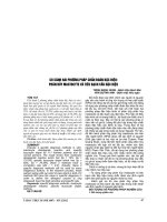
and normal breast tissue on mammograms [28, 115, 116]. The general architecture of

the CNN used in this study is shown in Figure 1.1. The input to the CNN is a regionof-interest (ROI) image, extracted for each of the potential signal sites. The nodes in
the hidden layers are arranged in groups, as are the weights associated with each node;
each weight group functions like a filter kernel. The CNN is trained to classify the input
ROI as containing a true microcalcification (TP) or a false signal (FP). In the implementation used in this study, the CNN had one input node, two hidden layers, and one
output node. All node groups in the two hidden layers were fully connected.
Training was performed with an error back propagation delta-bar-delta rule.
There were N1 node groups in the first hidden layer, and N2 node groups in the
second hidden layer. The kernel sizes of the first group of filters between the input
node and the first hidden layer were K1 × K1, and those of the second group of filters
between the first and second hidden layer were K2 × K2. For a CNN, learning is
constrained such that forward signal propagation is similar to a spatially invariant
convolution operation; the signals from the nodes in the lower layer are convolved
with the weight kernel, and the resultant value of the convolution is collected into
the corresponding node in the upper layer. This value is further processed by the
node through a sigmoidal activation function and produces an output signal that
will, in turn, be forward propagated to the subsequent layer in a similar manner. The
convolution kernel incorporates the neighborhood information in the input image
pattern and transfers the information to the receiving layers, thus providing the
pattern-recognition capability of the CNN.
The neural-network architecture used in many studies was selected using a
manual optimization technique [28] We evaluated the use of automated optimization
methods for selecting an optimal CNN architecture [117]. Briefly, three automated
Copyright 2005 by Taylor & Francis Group, LLC


2089_book.fm Page 8 Tuesday, May 10, 2005 3:38 PM

8

Medical Image Analysis

First
Hidden
Layer

Second
Hidden
Layer

K2

Output
Node

1
1

Input
ROI

•
•
•

K1

2

•
•
•

N2

N1

FIGURE 1.1 Schematic diagram of the architecture of a convolution neural network. The
input to the CNN is a region-of-interest (ROI) image extracted for each of the detected signals.
The output is a scalar that is the relative rating by the CNN representing the likelihood that
the input ROI contains a true microcalcification or a false-positive signal.

methods, the steepest descent (SD), the simulated annealing (SA), and the genetic
algorithm (GA) were compared. Four main parameters of the CNN architecture, N1,
N2, K1, and K2, were considered for optimization. The area under the ROC curve,
Az, [118] was used to design a cost function. The SA experiments were conducted
with four different annealing schedules. Three different parent selection methods
were compared for the GA experiments. The CNN was optimized with a set of ROI
images extracted from 108 mammograms. The suspected microcalcifications were
detected after the initial steps of the microcalcification-detection program [28]. The
detected signals were labeled as TP or FP automatically based on the ground truth
of the data set. A 16 × 16-pixel ROI centered at the signal site was extracted for
each of the detected locations, and these ROI images were used for training and
testing the CNN. The microcalcification-detection program detected more FP ROIs
than TP ROIs at the prescreening stage. For classifier training, it is more efficient
to have approximately equal numbers of TP and FP ROIs. Therefore, only a randomly
selected subset of FP ROI images was used. The selected ROIs were divided into
two separate groups, one for training and the other for monitoring the classification
accuracy of the trained CNN. Each group contained more than 1000 ROIs.
Another data set of 152 mammograms, which was different from the set of 108
mammograms employed for optimization of the CNN, was used for validation of
the detection program in combination with the CNN classifier. The optimal architecture

(N1-N2-K1-K2) was determined to be 14-10-5-7 using the training and validation
Copyright 2005 by Taylor & Francis Group, LLC


2089_book.fm Page 9 Tuesday, May 10, 2005 3:38 PM

Computer-Aided Diagnosis of Breast Cancer

9

sets. This optimal CNN architecture was then compared with the CNN architecture
of 12-8-5-3 determined by a manual search technique [28]. For comparison of the
performance of the CNN of different architectures, an independent data set of 472
digitized mammograms was used. This test data set was selected from the University
of South Florida (USF) digitized mammogram database, which is publicly available
over the Internet [119]. From the available cases in this database, only malignant
cases that were digitized with the Lumisys 200 laser scanner were selected (volumes:
cancer_01, cancer_02, cancer_05, cancer_09, and cancer_15). The data set contained
272 biopsy-proven microcalcification clusters, of which 253 were malignant and 19
were benign. There were 184 mammograms free of microcalcifications [119]. All
mammograms in the training, validation, and test sets were digitized at a pixel
resolution of 0.05 × 0.05 mm with 4096 gray levels. The images were converted to
0.1 × 0.1-mm resolution by averaging adjacent 2 × 2 pixels and subsampling. The
detection was carried out on the 0.1 × 0.1-mm resolution images.
1.2.1.5 False-Positive Reduction Using Clustering
A final step to reduce false positives is clustering. This approach is devised based
on clinical experiences that the likelihood of malignancy for clustered microcalcifications is generally much greater than sparsely scattered microcalcifications [102106]. Chan et al. [28, 113] designed a dynamic clustering procedure to identify
clustered microcalcifications. The image is initially partitioned into regions and the
number of potential signals in each region is determined. A region with a higher
concentration of potential signals is given a higher priority as a starting region to

grow a cluster. The cluster grows by searching for new members in its neighborhood
one at a time. A signal is included as a new member if it is within a threshold
distance from the centroid of the current cluster. The cluster centroid location is
updated after each new member is added. The cluster can grow across region
boundaries without constraints. Clustering stops when no more new members can
be found to satisfy the inclusion criteria. A cluster is considered to be true if the
number of members in the cluster is greater than a preselected threshold. The signals
that are not found to be in the neighborhood of any clusters will be considered
isolated noise points or insignificant calcifications and excluded. The specific parameters or thresholds used in the various steps depend on the spatial and gray level
resolutions of the digitized or digital mammograms [28, 113]. It was found that
having four detected signals within a clustering diameter of 1 cm provided a high
sensitivity for cluster detection.

1.2.2 FROC ANALYSIS

OF

DETECTION ACCURACY

The performance of a computer-aided detection system is generally evaluated by
the free-response receiver operating characteristic (FROC) analysis [120]. An FROC
curve shows the sensitivity of lesion detection as a function of the number of FPs
per image. In this study, it was generated by varying the input SNR threshold over
a range of values so that the detection criterion varied from lenient (low threshold)
to stringent (high threshold). After passing the size and contrast criteria, screening
by the trained CNN, and passing the regional-clustering criterion, the detected
Copyright 2005 by Taylor & Francis Group, LLC


2089_book.fm Page 10 Tuesday, May 10, 2005 3:38 PM

10

Medical Image Analysis

individual microcalcifications and clusters are compared with the "truth" file of the
input image. The number of TP and FP microcalcifications and the number of TP
and FP clusters are scored. The scoring method varies among researchers. In our
study, the detected signal was scored as a TP microcalcification if it was within 0.5
mm from a true microcalcification in the "truth" file. A detected cluster was scored
as a TP if its centroid coordinate was within a cluster radius (5 mm) from the centroid
of a true cluster and at least two of its member microcalcifications were scored as
TP. Once a true microcalcification or cluster was matched to a detected microcalcification or cluster, it would be eliminated from further matching. Any detected
microcalcifications or clusters that did not match to a true microcalcification or
cluster were scored as FPs. The trade-off between the TP and FP detection rates by
the computer program was analyzed as an FROC curve. A low SNR threshold
corresponded to a lax criterion with high sensitivity and a large number of FP
clusters. A high SNR threshold corresponded to a stringent criterion with a small
number of FP clusters and a loss in TP clusters. The detection accuracy of the
computer program with and without the CNN classifier could then be assessed by
comparison of the FROC curves.
To test the performance of the selected optimal architecture, the detection program was run at seven SNR threshold values varying between 2.6 and 3.2 at
increments of 0.1. Figure 1.2a shows the FROC curves of the microcalcificationdetection program using both the manually optimized and automatically optimized
CNN architectures. The FP rate was estimated from the computer marks on the 184
normal mammograms that were free of microcalcifications in the USF data set. The
automatically optimized architecture outperformed the manually optimized architecture. At an FP rate of 0.7 cluster per image, the film-based sensitivity is 84.6%
with the optimized CNN, in comparison with 77.2% for the manually selected CNN.
Figure 1.2b shows the FROC curves for the microcalcification-detection programs
if clusters having images in both CC and MLO views are analyzed and a cluster is
considered to be detected when it is detected in one or both views. This “case-based”

scoring has been adopted for the evaluation of some CAD systems [20]. The rationale
is that if the CAD system can bring the radiologist’s attention to the lesion on one
of the views, it will be unlikely that the radiologist will miss the lesion. For casebased scoring, the sensitivity at 0.7 FPs/image is 93.3% for the automatically optimized CNN and 87.0% for the manually selected CNN. This study demonstrates
that classification of true and false signals is an important step in the microcalcification-detection program and that an optimized CNN can effectively reduce FPs and
improve the detection accuracy of the CAD system.
An automated optimization algorithm such as simulated annealing can find the
optimum more efficiently [117, 121–123] than a manual search, which may find
only a local optimum because it is difficult to explore adequately a high-dimensional
parameter space. The optimization described here is applied to one stage, FP reduction with the CNN, of the detection program. The cost function was based on the
Az of the CNN classifier for its performance in differentiating the TP and FP signals.
Ideally, one would prefer to optimize all parameters in the detection program
together. In such a case, optimizing the performance in terms of the FROC curve
will be necessary. The principle of optimizing the entire detection system is similar
Copyright 2005 by Taylor & Francis Group, LLC


2089_book.fm Page 11 Tuesday, May 10, 2005 3:38 PM

Computer-Aided Diagnosis of Breast Cancer

11

0.95

TP Fraction

0.90

0.85

0.80

0.75
Manual optimization
Automatic optimization
0.70
0.0

0.5

1.0

1.5
2.0
2.5
No. of FP Marks per Image

3.0

3.5

4.0

(a)
0.95

TP Fraction

0.90

0.85

0.80

0.75
Manual optimization
Automatic optimization
0.70
0.0

0.5

1.0

1.5
2.0
2.5
No. of FP Marks per Image

3.0

3.5

4.0

(b)

FIGURE 1.2 Comparison of test FROC curves for detection of clustered microcalcifications
with manually optimized CNN architecture (12-8-5-3) and automatically optimized CNN
architecture (14-10-5-7): (a) film-based (single view) scoring and (b) case-based (CC and

MLO views) scoring. The evaluation was performed using a test data set with 472 images.

to that of optimizing the TP-FP classifier, except that a proper cost function has to
be designed to guide the optimization.
It may be noted that we discuss here a three-stage (training-validation-test)
methodology for development and evaluation of CAD system performance. This
Copyright 2005 by Taylor & Francis Group, LLC


2089_book.fm Page 12 Tuesday, May 10, 2005 3:38 PM

12

Medical Image Analysis

methodology requires separate data sets for each stage. The training data set is used
to select the sets of parameters for the neural network architecture and neural network
weights. The validation set is used to evaluate the performance of the selected
architectures and identify the architecture with the best performance. Once the
architecture is selected using the validation set, the parameters of the detection
program are fixed, and no further changes should be made. The performance of the
program is then evaluated with an independent test set. The images in this set were
used only to assess the performance of the fully specified optimal architecture. If
only a small training set and an “independent” test set are used, and the detection
performance on the test set is used as a guide to adjust the parameters of the detection
program, there is always a bias due to fine-tuning the CAD system to this particular
“test” data set that is essentially a validation set. The results achieved with that test
set may not be generalizable to other data sets. This is an important consideration
for CAD system development. Before a CAD system can be considered for clinical
implementation, it is advisable to follow this three-stage methodology and to evaluate

the system with an independent random test set that contains a large number of cases
with a wide spectrum of characteristics. Otherwise, the test results may not reflect
the actual performance of the CAD program in the unknown patient population.

1.2.3 EFFECTS OF COMPUTER-AIDED DETECTION
RADIOLOGISTS’ PERFORMANCE

ON

One of the important steps in the development of a CAD system is to evaluate
whether the computer’s opinion has any impact on radiologists’ performance. ROC
methodology is a well-known approach to comparing two diagnostic modalities.
The important issues involved in the design of ROC experiments can be found in
the literature [118]. We will describe as an example an observer ROC study to
evaluate the effects of a computer aid on radiologists’ accuracy in the detection of
microcalcifications with and without aid [18].
In the ROC study, a set of 60 mammograms, half of which were normal and the
other half of which contained very subtle microcalcifications, was used. The accuracy
of the microcalcification-detection program at the time of the study was 87% at 4
FPs/image for this data set. A simulated detection accuracy of 87% at 0.5 FPs/image
was also included in the ROC experiment to evaluate the effect of FPs on radiologists’
detection. Seven attending radiologists and eight radiology residents participated as
observers. They read the mammograms under three different conditions: one without
CAD, the second with CAD having an accuracy of 87% at 4 FPs/image, and the
third condition with CAD having an accuracy of 87% at 0.5 FPs/image. The reading
for each observer was divided into three sessions, and the reading order of the
radiologists using the three conditions was counterbalanced so that no one condition
would be read by the observers in a given order more often than the other two
conditions. The observers were asked to use a five-point confidence rating scale to
rate their confidence in detecting a microcalcification cluster in an image. The

confidence rating scale was analyzed by ROC methodology.
The ROC curves obtained from the observer experiment are shown in Figure
1.3. The average sensitivity over the entire range of specificity is represented by the
Copyright 2005 by Taylor & Francis Group, LLC


2089_book.fm Page 13 Tuesday, May 10, 2005 3:38 PM

Computer-Aided Diagnosis of Breast Cancer

13

1.0

True-positive Fraction

0.8

0.6

0.4

0.2

without CAD (Az = 0.94)
with CAD-L1 (Az = 0.97)
with CAD-L2 (Az = 0.98)

0.0
0.0

0.2

0.4
0.6
False-positive Fraction

0.8

1.0

FIGURE 1.3 Comparison of the average ROC curves for detection of microcalcifications
with and without CAD. L1 is the computer performance level of 87% sensitivity at 4 FPs/
per image, and L2 is the simulated computer performance level of 87% sensitivity at 0.5 FPs/
per image. The average ROC curves were obtained by averaging the slope and intercept
parameters of the individual ROC curves from the 15 observers. The improvement in the
detection accuracy, Az, was statistically significant at p < 0.001 for both CAD conditions.

area under the ROC curve, Az. It was found that the Az improved significantly (p <
0.001) when the radiologists read the mammograms with the computer aid, either
at 0.5 FPs/image or at 4 FPs/image, compared with when they read the mammograms
without the computer aid. Although the Az of the CAD reading with 0.5 FPs/image
was slightly higher than that with 4 FPs/image, the difference did not achieve
statistical significance, indicating that the observers were able to discard FPs detected
by the computer. This ROC study was the first experiment to demonstrate that CAD
has the potential to improve breast cancer detection, thus establishing the significance
of CAD research in mammography.

1.3 COMPUTERIZED DETECTION OF MASSES
Mass is another major sign of breast cancer. Masses are imaged as focal density on

mammograms. In mammograms of fatty breasts, a dense mass — low-optical-density
(white) region surrounded by a darker gray background — can easily be detected
by radiologists. However, in most breasts there is fibroglandular tissue that also
appears as dense white regions on mammograms, and this camouflaging effect makes
it difficult for radiologists to detect the masses. There are several major types of
masses, as described by the characteristics of their borders, including well-circumscribed, ill-defined, and spiculated. Masses with well-circumscribed margins are
more likely to be benign cysts or fibroadenomas, whereas masses with ill-defined
Copyright 2005 by Taylor & Francis Group, LLC


2089_book.fm Page 14 Tuesday, May 10, 2005 3:38 PM

14

Medical Image Analysis

or spiculated borders have a high likelihood of being malignant. Some CAD
researchers designed their mass-detection programs making use of the border characteristics of spiculated masses [19, 52, 55, 64, 65, 68]. Karssemeijer et al. employed
statistical analysis to develop a multiscale map of pixel orientations. Two operators
sensitive to radial patterns of straight lines were constructed from the pixel-orientation map. The operators were then used by a classifier to detect stellate patterns
in the mammogram [64]. Kobatake et al. used line skeletons and a modified Hough
transform to detect the spicules, which are radiating line structures extending from
the mass [65, 68]. Finally, Ng et al. used a spine-oriented approach to detect the
microstructure of mass spicules [55].
Since a substantial fraction of nonspiculated masses are malignant, detection of
nonspiculated masses is as important as detecting spiculated masses. A number of
mass-detection algorithms were developed to detect masses without focusing on
specific border characteristics [52, 54, 56–63, 66, 67, 69–71]. Most of the massdetection programs were applied to a single-view mammogram. The mammogram
is first preprocessed with a filter or nonlinear technique to enhance the suspicious
regions. The potential signals are segmented from the background based on morphological and gray-scale information. Feature descriptors are extracted from the

segmented signals. Rule-based classifiers or other linear, nonlinear, or neural-network classifiers are then trained to classify the signal candidates as true mass or
false positives.
Laine et al. applied multiscale wavelet analysis to enhance contrast of a mammogram [58, 60]. Petrick et al. used adaptive enhancement, region growing, and
feature classification to detect suspicious mass regions in a mammogram [63, 70,
124]. Li et al. employed a modified Markov random field model and adaptive
thresholding to segment regions in an image [59]. A fuzzy binary-decision-tree
classifier then classified the regions as suspicious or normal. Zheng et al. used
Gaussian band-pass filtering to detect suspicious regions and rule-based multilayer
topographic-feature analysis to classify the regions [61]. Guliato et al. proposed a
fuzzy region-growing method for mass detection [66].
Radiologists often used the approximate symmetry in the distribution of dense
tissue in the left and right breasts of a patient to detect abnormal growth. Yin et al.
developed a mass-detection method based on this information. Their technique,
bilateral subtraction, subtracted corresponding left and right mammogram after the
two images were aligned. Morphological and texture features were then extracted
from the detected regions to decrease the number of FP detections [54, 56]. Another
important technique used by radiologists in mammographic interpretation is to
compare current and prior mammograms to detect new density or changes in the
existing densities. Computer vision techniques for comparing current with prior
mammograms have been proposed. Brzakovic et al. registered the current and prior
mammograms using a principal-axis method. The mammograms were then partitioned using hierarchical region growing and compared using region statistics [57].
Sanjay-Gopal et al. [96] developed a regional-registration technique in which the
mammograms were aligned based on maximizing mutual information between the
breast regions on the two images. Polar coordinate systems, based on the nipple and
breast centroid locations, were established for both images. The center of the lesion
Copyright 2005 by Taylor & Francis Group, LLC


2089_book.fm Page 15 Tuesday, May 10, 2005 3:38 PM

Computer-Aided Diagnosis of Breast Cancer

15

on the current image was then transformed to the prior image. A fan-shaped region,
based on the polar coordinate system and centered at the centroid of the lesion, was
defined and searched to obtain a final estimate of the mass location in the prior
image. Hadjiiski et al. [125, 126] further improved the accuracy of the regionalregistration technique by incorporating a local search method to refine the lesion
location. Local search was guided by simplex optimization and a correlation similarity measure. Radiologists routinely use two-view (CC and MLO views) mammograms for lesion detection. Paquerault et al. [100] developed a mass-detection
method that fuses the detection on the CC and MLO views to reduce false positives.
They demonstrated that the two-view fusion method can improve the detection
accuracy for masses on mammograms.
In this section, we will discuss our approach as an example of an automated
technique for detection of masses using one-view information. A two-view information-fusion technique is discussed in the next section.

1.3.1 METHODS
We have developed a mass-detection program for single-view mammograms. The
method is based on the information that masses manifest as density on mammograms. It does not presuppose certain shape, size, or border properties for a mass
and thus is designed to detect any type of masses.
The block diagram for our mass-detection scheme is shown in Figure 1.4. This
scheme combines adaptive enhancement with local object-based region-growing and
feature-classification techniques for segmentation and detection. We developed a
density-weighted contrast enhancement (DWCE) filter as a preprocessing step. The
DWCE filter enhances the contrast between the breast structures and the background
Input mammogram

DWCE enhancement

Object refinement

Rule-based FP reduction

Overlap reduction

Texture feature analysis

Detected objects

FIGURE 1.4 Block diagram for the mass-detection scheme.
Copyright 2005 by Taylor & Francis Group, LLC


2089_book.fm Page 16 Tuesday, May 10, 2005 3:38 PM

16

Medical Image Analysis

based on the local breast density. Suspicious structures on the enhanced breast image
are identified. Each of the identified structures is then used as the seed point for
object-based region growing. The region-growing technique uses gray-scale information to segment the object borders and to reduce merging between adjacent or
overlapping structures. Morphological and texture features are extracted from the
grown objects. Rule-based classification and a classifier using linear discriminant
analysis (LDA) are used to distinguish breast mass or normal structures based on
the extracted features. In order to reduce the large number of initial structures, a
first-stage rule-based classifier, based on morphological features, is used to eliminate
regions whose shapes are significantly different from breast masses. A second-stage
classifier was trained to select useful features and merge them to form a linear
discriminant that makes a final decision to distinguish between true masses and
normal structures.

1.3.1.1 Preprocessing and Segmentation
We designed an adaptive filter to enhance the dense structures on digital mammograms. Because most mass lesions have blurred borders, and because commonly
used edge-enhancement methods cannot sharpen the mass margins very well, the
low-contrast dense breast structures are first enhanced by a nonlinear filter using an
enhancement factor that is weighted by the local density [62]. A Laplacian-Gaussian
(LG) edge detector is then applied to the enhanced structures to extract the object
boundaries. The adaptive filter is an expansion of the adaptive contrast and mean
filter of Peli and Lim [127]. The block diagram for the enhancement filter is shown
in Figure 1.5. The mammogram is first filtered to derive a contrast image and a
density image, IC(x, y) and ID(x, y), respectively. The contrast image is weighted by
a multiplication factor that depends on the local value of the density image. Finally,

I(x, y)

Band-pass filtered
IC (x, y)

Low-pass filtered
ID (x, y)

WD (⋅)
X

W (⋅)

IE (x, y)

FIGURE 1.5 Block diagram for the DWCE filter.
Copyright 2005 by Taylor & Francis Group, LLC

2089_book.fm Page 17 Tuesday, May 10, 2005 3:38 PM

Computer-Aided Diagnosis of Breast Cancer

17

the weighted contrast image undergoes a nonlinear pixelwise transformation to
generate the final “enhanced” image. The two-step DWCE filtering is described as

( )

( ( )) ( )

I W x, y = WD I D x, y ⋅ I C x, y

( )

( ( ))

I E x, y = W I W x, y

(1.1)
(1.2)

The multiplication factor and the nonlinear transformation function used in this
application, WD(⋅) and W(⋅), can be found in the literature [62]. The DWCE filter
suppresses very low-contrast regions, emphasizes low- to medium-contrast regions,
and slightly suppresses the high-contrast regions. The suppression of very lowcontrast regions reduces bridging between adjacent breast structures. The enhancement of low- to medium-contrast regions accentuates the subtle structures that
contain most of the mammographic masses. The slight suppression of the highcontrast regions results in a more uniform intensity distribution of the breast structures. After DWCE filtering, the mammogram should have a relatively uniform

background superimposed with enhanced breast structures that can be segmented
with Laplacian-Gaussian edge detection [128, 129]. The regions enclosed by the
detected edges are considered to be mass candidates.
1.3.1.2 Object Refinement
Although the DWCE filtering with LG edge detection can extract breast structures
including most of the masses, the borders of the objects are not close to the true
object border. The detected object borders are generally within the true object borders
because of our attempt to minimize merging between structures. However, many
adjacent objects are still found to merge together. The next stage of the massdetection program is designed to refine the object borders and to separate the merged
objects. The object-refinement stage is needed before extraction of morphological
and texture features to distinguish true mass and normal breast structures. The
purpose of the local refinement stage is to improve the accuracy of object borders
found by the DWCE segmentation.
For refinement of the objects, seed locations are first identified by finding the
local maxima within each object detected in the DWCE stage. The local maxima
are determined using the ultimate-erosion technique [130]. These local maxima are
then grown into seed objects by using Gaussian smoothing σ = 0.4 mm. Each seed
object is further grown by selecting all connected pixels with gray values in the
range Mi ± 0.01Mi , where Mi is the gray level of the ith local maximum. K-means
clustering is then applied to a 25 × 25-mm background-corrected ROI [116] centered
on each seed object to refine the initial object border [131]. The background correction method described by Sahiner et al. was used to estimate the low-frequency
background of the ROI [116]. The pixel value of a given pixel on the background
image is estimated as the weighted sum of the four pixel values along the edges of
the ROI intersecting with a horizontal line and a vertical line passing through the
given pixel. The weight for an edge pixel is inversely proportional to the distance
Copyright 2005 by Taylor & Francis Group, LLC


2089_book.fm Page 18 Tuesday, May 10, 2005 3:38 PM

18

Medical Image Analysis

from the given pixel to the edge pixel. The estimated background image is subtracted
from the ROI to reduce the background variation before K-means clustering.
For the K-means clustering, each pixel in the ROI is represented by a feature
vector Fi in a multidimensional feature space. In this application, the feature vector
is composed of two components: the gray level and a median filtered value (median
filter kernel = 1 × 1 mm) of the pixel. The clustering algorithm [132, 133] assigns
the class membership of the feature vector Fi of each pixel in an iterative process.
The algorithm first chooses the initial cluster center vectors, Co and Cb for the object
and the background, respectively. For each feature vector Fi, the Euclidean distance
do(i) between Fi and Co, and the Euclidean distance db(i) between Fi and Cb are
calculated. If the ratio db(i)/do(i) is larger than a predetermined threshold R, then
the vector is temporarily assigned to the group of object pixels; otherwise, it is
temporarily assigned to the group of background pixels. Using the new pixel assignments, a new object-cluster center vector and a new background-cluster center vector
are computed as the mean of the vectors temporarily assigned to the group of object
pixels and to the group of background pixels, respectively. This completes one
iteration of the clustering algorithm. The iterations continue until the new and old
cluster center vectors are the same or the changes are less than a chosen value, which
means that the class assignment for each pixel has converged to a stable value. The
clustering process does not guarantee connectivity of the pixels assigned to the same
class. Therefore, several disconnected objects may be generated in an ROI after
clustering, and the object may have holes. The holes within the objects are filled,
and the largest connected object among all detected objects in the ROI is selected
as the object of interest. Figure 1.6 shows an example of a mammogram demonstrating the DWCE-extracted regions and the detected objects before and after
clustering is applied.

(a)

(b)

(c)

(d)

FIGURE 1.6 Example of local object refinement and detection: (a) objects initially detected
by DWCE at 800 µm resolution, (b) original mammogram with two of the ROIs; the upper
one is normal breast tissue, the lower one is a true mass. (c) the DWCE segmented objects
in each ROI, and (d) the final objects after clustering and filling. The true mass and one FP
are the detected objects at the output of the system.
Copyright 2005 by Taylor & Francis Group, LLC


2089_book.fm Page 19 Tuesday, May 10, 2005 3:38 PM

Computer-Aided Diagnosis of Breast Cancer

19

1.3.1.3 Feature Extraction and Classification
The initial objects from the prescreening DWCE stage include a large number of
normal breast structures (false positives). In order to overcome the problems associated with the large number of objects, we perform the feature classification in two
stages. Eleven morphological features are initially used with a threshold and a linear
classifier to remove detected normal structures that are significantly different from
breast masses. Texture-based classification then follows this morphological-reduction stage. Fifteen global and local multiresolution texture features, based on the
spatial gray-level dependence (SGLD) matrices are used as inputs to an LDA classifier, which merges the input feature into a single discriminant score for each
detected object. Decision thresholds based on this score and on the maximum number
of marks allowed per image are then used to identify potential breast masses. These

feature-extraction and classification steps are described briefly below. Further details
can be found in the literature [62, 70, 73, 86, 134].
We extracted a number of morphological features from the segmented objects.
Eleven of these features are selected for the initial differentiation of the detected structures [63, 70]. Ten of these features are based solely on the binary-object shape extracted
by the segmentation. Five of the ten are based on the normalized radial length (NRL).
NRL is defined as the Euclidean distance from the centroid of an object to each of its
edge pixels and normalized relative to the maximum radial length for the object [74].
The NRL features include the mean, standard deviation, entropy, area ratio, and zero
crossing count. The six other morphological features are: number of perimeter pixels,
area, perimeter-to-area ratio, circularity, rectangularity, and contrast [70]. The morphological features are used as input variables to a rule-based classifier followed by an
LDA classifier. The rule-based classification sets a maximum and minimum value for
each morphological feature based on the maximum and minimum feature values found
for the breast masses in the training set. The remaining objects after rule-based classification are input to a trained LDA classifier that merges the feature values into a
discriminant score. A threshold chosen during training is then applied to the output
score to distinguish true masses from normal breast structures.
After classification of morphological features, another classifier based on texture
features is applied [63, 70, 135, 136]. First, a set of multiresolution texture features
is extracted from 100-µm resolution mammograms. The ROIs have a fixed size of
256 × 256 pixels, and the center of each ROI corresponds to the centroid location
of a detected object. If the object is located near the border of the breast and a
complete 256 × 256-pixel ROI cannot be defined, the ROI is shifted until it is entirely
inside the breast area and the appropriate edge coincides with the border of the
original mammogram. For a given ROI, background correction is first performed to
reduce the low-frequency gray-level variation due to the density of the overlapping
breast tissue and the X-ray exposure conditions, as described previously for the Kmeans clustering. A more detailed description of this background correction method
can be found in the literature [116, 137]. The estimated background image is
subtracted from the original ROI to obtain a background-corrected image.
Global and local multiresolution texture features derived from the SGLD matrices of the background-corrected ROI are used in texture analysis. The SGLD matrix
element, pθ,d(i, j), is the joint probability of the occurrence of gray levels i and j for

Copyright 2005 by Taylor & Francis Group, LLC


2089_book.fm Page 20 Tuesday, May 10, 2005 3:38 PM

20

Medical Image Analysis

pixel pairs that are separated by a distance d and at a direction θ [138]. In a previous
study, we did not observe a significant dependence of the discriminatory power of
the texture features on the direction of the pixel pairs for mammographic textures
[137]. However, since the actual distance between the pixel pairs in the diagonal
direction was a factor of 2 greater than that in the axial direction, the feature
values in the axial directions (0° and 90°) and in the diagonal directions (45° and
135°) were grouped separately for each texture feature derived from the SGLD
matrix at a given pixel-pair distance.
Thirteen texture measures are derived from each SGLD matrix, including correlation, entropy, energy (angular second moment), inertia, inverse difference
moment, sum average, sum entropy, sum variance, difference average, difference
entropy, difference variance, information measure of correlation 1, and information
measure of correlation 2. The formulation of these texture measures can be found
in the literature [43, 138]. To extract texture features, individual ROIs are first
decomposed into different scales by using the wavelet transform with a four-coefficient Daubechies kernel. For global texture features, 4 wavelet scales, 14 interpixel
distances d, and 2 directions (axial and diagonal) are used to produce 28 different
SGLD matrices. A total of 364 global multiresolution texture features are thus
calculated for each ROI. To further describe the information specific to the mass
and its surrounding normal tissue, a set of local texture features are derived from
subregions of each ROI [63, 136, 139]. Five subregions, including an object region
with the detected object in the center and four peripheral regions at the corners, are
segmented from each ROI. A total of 104 local texture features are calculated from

the eight SGLD matrices (4 interpixel distances × 2 angles × 13 texture features) of
the object region. Another 104 local texture features are derived from the eight SGLD
matrices of the periphery regions. The final set of local textures includes the 104
features from the object region and an additional 104 features derived as the difference between the corresponding features in the object and the periphery. The total
number of global and local texture features is 572. Because the generalizability of
classifiers usually degrades with increased dimensionality of the feature space, a
stepwise feature-selection procedure is applied to the feature space to select a small
subset of features that are effective for the classification task.
The stepwise LDA is a commonly used method for selection of useful feature
variables from a large feature space. Details on the application of stepwise feature
selection can be found in the literature [135, 137, 140]. Briefly, stepwise LDA uses
a forward-selection and backward-removal strategy. When a feature is entered into
or removed from the model, its effect on the separation of the two classes can be
analyzed by one of several criteria. We use the Wilks's lambda criterion, which
minimizes the ratio of the within-group sum of squares to the total sum of squares
of the two class distributions. The significance of the change in the Wilks's lambda
is estimated by F-statistics. In the forward-selection step, the features are entered
one at a time. The feature variable that causes the most significant change in the
Wilks's lambda is included in the feature set if its F value is greater than the F-toenter (Fin) threshold. In the feature-removal step, the features already in the model
are eliminated one at a time. The feature variable that causes the least significant
change in the Wilks's lambda is excluded from the feature set if its F value is below
Copyright 2005 by Taylor & Francis Group, LLC


2089_book.fm Page 21 Tuesday, May 10, 2005 3:38 PM

Computer-Aided Diagnosis of Breast Cancer

21

the F-to-remove (Fout) threshold. The stepwise procedure terminates when the F values
for all features not in the model are smaller than the Fin threshold and the F values for
all features in the model are greater than the Fout threshold. The number of selected
features decreases if either the Fin threshold or the Fout threshold is increased. Therefore,
the number of features to be selected can be adjusted by varying the Fin and Fout values.
The selected texture features are used as input predictor variables to formulate
an LDA classifier. A threshold-discriminating score is used to differentiate between
true masses and false positives. In this implementation, all scores in an individual
image are scaled before thresholding so that the minimum score in the image is 0
and the maximum score is 1. This scaling minimizes the nonuniformity seen between
mass structures in different images. It also results in at least one structure being
detected in each image.

1.3.2 FROC ANALYSIS

OF

DETECTION ACCURACY

1.3.2.1 Data Sets
A database of mammograms with known truth is needed for training and testing of
CAD algorithms. The ground truth of each case used in the following study was
based on biopsy results, and the true mass location was identified by radiologists
experienced in mammographic interpretation.
1.3.2.1.1 Training Set
The clinical mammograms used for training the algorithm parameters, referred to
as the training cases, were selected from the files of patients who had a mammographic evaluation and biopsy at our institution. In our clinical practice, a multiplereading paradigm with a resident or fellow previewing each case followed by an
official interpretation by an attending radiologist was typically followed during the
initial evaluation of each case. The mammograms were acquired with Kodak
MinR/MinR or MinR/MRE screen/film systems using dedicated processing. Series

of consecutive malignant and consecutive benign mass cases were collected using
a computerized biopsy registry. The selection criterion was that a biopsy-proven
mass existed on the mammogram. No case-selection bias was used except for the
exclusion of microcalcifications cases without a visible mass, architectural distortion
cases, and mass cases containing masses larger than 2.5 cm. The data set consisted
of 253 mammograms from 102 patients examined between 1981 and 1989. The
training set included 128 malignant and 125 benign masses. Sixty-three of the
malignant and six of the benign masses were judged to be spiculated by a radiologist
qualified by the Mammography Quality Standards Act (MQSA). The mammograms
were digitized with a Lumisys DIS-1000 laser film scanner with a pixel size of 100µm and 12-bit gray-level resolution. The gray levels were linearly proportional to
optical density in the 0.1- to 2.8-optical density unit (O.D.) range and gradually fell
off in the 2.8- to 3.5-O.D. range.
1.3.2.1.2 Independent Test Set
The performance of a trained CAD algorithm has to be evaluated with independent
cases not used for training. Cases were collected from two different institutions and
Copyright 2005 by Taylor & Francis Group, LLC


2089_book.fm Page 22 Tuesday, May 10, 2005 3:38 PM

22

Medical Image Analysis

were not used in the training process. Series of consecutive malignant- and consecutive benign-mass cases were collected using a biopsy registry from each institution,
in a manner similar to the training-case collection process.
The first set of preoperative cases, referred to as Group 1, was selected from the
files of 127 patients who had a mammographic evaluation and biopsy at our institution between 1990 and 1999. The Group 1 case came from the same institution
as the training cases and contained at least one proven breast mass visible with
mammography. Again, a resident or fellow typically previewed each Group 1 case

followed by an official interpretation by an attending (prior to MQSA in 1994) or
an MQSA radiologist during the initial evaluation of these cases. Each case consisted
of a single CC and either an MLO or lateral view of the breast containing the mass.
For simplicity, we will refer to all views other than the CC view as the MLO view
in the following discussions, with the understanding that this also includes some
lateral views. If both breasts of a patient had a mass, each breast was considered to
be an independent case. Using this breast-based definition, a total of 138 cases (276
mammograms) were available. The mammograms were acquired with Kodak
MinR/MRE screen/film systems using dedicated processing in the years prior to
1997 (154 mammograms) and a Kodak MinR 2000 screen/film system from 1997
on (122 mammograms). Each case contained one or more preoperative breast masses
that were identified prospectively during initial clinical evaluation or mammographic
interpretation. The independent Group 1 mammograms were digitized with a Lumisys LS 85 laser film scanner at 50-µm and 12-bit gray-level resolution. The gray
levels were calibrated to be linearly proportional to optical density in the 0.1- to
4.0-O.D. range. The images were reduced to a 100-µm pixel size by averaging 2 × 2pixel neighborhoods before performing mass detection.
Clinical cases from the public database available from the University of South
Florida (USF) were also analyzed [119]. We evaluated 142 CC/MLO pairs from 136
patients collected by USF between 1992 and 1998. Each USF case contained at least
one proven breast mass visible on mammography. Additional information on the
USF database can be found in the literature [119]. For compatibility with the Group
1 database, we only selected USF cases digitized with a Lumisys 200 laser film
scanner. This scanner again digitized the images at 50-µm and 12-bit gray-level
resolution, but the gray levels were calibrated to be linearly proportional to optical
density in the 0.1- to 3.6-O.D. range. In the following discussions, these 142 USF
cases that came from a different institution than the training cases are referred to as
the Group 2 cases.
Lesion-free mammograms of the breast contralateral to a breast containing an
abnormality were used to estimate the CAD marker rate for the algorithm. These
mammograms are referred to as normal cases in this study. A mammogram was
regarded as normal if it did not contain a visible mass during the time of the

mammographic exam and upon second review by an MQSA radiologist during data
collection. A total of 251 mammograms from the 127 Group 1 patients and 252
mammograms from the 136 Group 2 patients were included as normal cases. There
were fewer normal than abnormal mammograms because not all of the contralateral
mammograms were digitized, and 7 of the 263 combined Group 1 and Group 2
patients had visible lesions in both the right and left breasts.
Copyright 2005 by Taylor & Francis Group, LLC


2089_book.fm Page 23 Tuesday, May 10, 2005 3:38 PM

Computer-Aided Diagnosis of Breast Cancer

23

Table 1.1 summarizes the Group 1 and 2 test cases used to evaluate the massdetection algorithm. It includes the number of malignant and benign masses separated by whether they were visible in both views or only in a single view. The
mammographic size for the Group 1 masses was measured by the radiologist during
initial case evaluation. The malignant Group 1 masses had a mean size, standard
deviation, and median size of 15.4 mm, 12.0 mm, and 12.0 mm, respectively. The
benign Group 1 masses had a mean size, standard deviation, and median size of
13.4 mm, 11.8 mm, and 10.0 mm, respectively. Radiologist-measured mass sizes
were not available for the Group 2 cases because we found that the boundary of the
masses, hand-drawn by the reviewing radiologists, were much larger than the actual
mammographic lesion size. Therefore, mass size information is not reported for the
Group 2 cases.
1.3.2.2 True Positive and False Positive
One important consideration in the evaluation of the performance of a CAD algorithm is the definition of the TPs and FPs. Even if the algorithm is fixed, the reported
detection sensitivity and specificity have been found to be dependent on these
definitions. For the Group 1 cases, the smallest bounding box containing the entire
mass identified by a radiologist was used as the truth. For Group 2, we used a

bounding box around the radiologist-outlined mass region provided with each image.
Our definition of a TP was based on the percentage of overlap between the bounding
box of an identified structure and the bounding box of the true mass. Based on the
training set, we chose an overlap threshold of 25%. This value corresponds to the
minimum overlap between the bounding box of a detected object and the bounding
box of a true mass for the object to be considered a TP detection. The 25% threshold
was selected because it was found to match well with TPs identified visually. The
detected objects were first labeled automatically by the computer using this criterion.
All of the TPs were then visually reviewed to make sure that the program highlighted
the true lesion and not a neighboring structure. Marks that were found to match
neighboring structures were considered to be FPs.
The number of FP marks produced by the algorithm was determined by counting
the markings produced in normal cases. We used a total of 251 normal mammograms
from Group 1 and 252 normal mammograms from Group 2 to estimate the marker
rate. The true-positive fraction (TPF) or sensitivity, calculated from the abnormal
cases, and the average number of marks per image, calculated from the normal cases,
were determined for a fixed set of thresholds at the final texture-classification stage.
The TPF and the average number of marks per mammogram as the decision threshold
varied were then used to plot the FROC performance curves for malignant and
benign masses in the different data sets.
1.3.2.3 Training and Testing
The computer program was trained using the entire training data set of 253 mammograms. This included adjusting the filters, clustering, selected features, and classification thresholds. Once training was completed, the parameters and all thresholds
Copyright 2005 by Taylor & Francis Group, LLC


Abnormal
Malignant
Total
Mammograms

Patients

One-View
Masses

Group 1
Group 2

276
284

127
136

2
5

Individual Masses
72
96

Group 1
Group 2

128
184

64
92

—
—

Grouped Masses
64
92

Database

Two-View
Masses

Benign
One-View
Masses

Normal

Two-View
Masses

Mammograms

Patients

3
6

78
63

251
252

93
128

—
—

—
—

251
252

93
128

Medical Image Analysis

Note: One-view masses correspond to masses visible in only one mammographic view in the pair; two-view masses correspond to
masses visible in both mammographic views in the pair. The individual-masses category considers each mass in a mammogram or case
as a TP during scoring; the grouped-masses category considers all malignant masses for a mammogram or case together as one TP
during scoring.

2089_book.fm Page 24 Tuesday, May 10, 2005 3:38 PM

24

Copyright 2005 by Taylor & Francis Group, LLC

TABLE 1.1
Summary of Cases, Patients, and Masses in Group 1 and Group 2 Databases


2089_book.fm Page 25 Tuesday, May 10, 2005 3:38 PM

Computer-Aided Diagnosis of Breast Cancer

25

were fixed for testing. The training data set was then resubstituted into the algorithm
and was found to have an image-based (i.e., each mass on each mammogram was
considered as an independent sample) training sensitivity of 81% (85% for malignant
masses), with 2.9 marks per mammogram on average at this sensitivity level. It is
important to note that the detection classifiers considered only classification between
breast masses and normal tissue, and not between malignant and benign masses.
Therefore, no distinction was made between malignant and benign masses in the
training process.
1.3.2.4 Performance of Mass Detection Algorithm
The detection performance of a CAD algorithm for mammography can be analyzed
on a per-mammogram or per-case basis. In the former, the CC and MLO views are
considered independently, so that a lesion visible in the CC view is considered as a
TP, and the same lesion in the MLO view is a different TP. In the latter case, a mass
is considered to be detected if it is detected on either the CC view, the MLO view,
or on both views. The latter evaluation takes into consideration that, in clinical
practice, once the computer alerts the radiologist to a cancer in one view, it is unlikely
that the radiologist will miss the cancer. The per-case approach is often used by
researchers in reporting their CAD performance [20, 141, 142]. Results are also

presented for two different TP scoring methods. The individual scoring method
considers each mass in a mammogram or case as a different TP. The grouped scoring
method considers all malignant masses in a mammogram or case as a single TP
[20]. The rationale for group scoring is that a radiologist might not need to be alerted
to all malignant lesions in a mammogram or case before taking action. Therefore,
multiple detections in a mammogram or case might not significantly enhance the
power of CAD. These different definitions of computer detection are included here
to illustrate the dependence of performance on the scoring methods. It is therefore
important to clearly define the scoring method in reporting or comparing performance of CAD algorithms.
FROC performance curves based on individual mass scoring for the Group 1
cases are shown in Figure 1.7. Similar data are presented for the Group 2 cases in
Figure 1.8. These figures include per-case and per-mammogram performance curves
for the detection of both the malignant and benign masses, and these are included
to show the TPF achievable for a large range of marker rates. It can be seen that
the performance for the Group 2 benign cases is much lower than that for the Group
1 benign cases. However, the difference in performance between the Group 1 and
Group 2 malignant masses is small.
The per-case and per-mammogram FROC performance curves for malignant
masses based on grouped-mass scoring is shown in Figure 1.9. These curves show
how TPF varies as a function of marker rate based on group scoring, which is
expected to be the best clinically relevant measure of algorithm performance. It is
evident from the curves that the algorithm provides consistent malignant mass-detection
performance for both independent test sets over a wide range of marker rates.
In the Group 1 database, 34% (49/146) of the malignant and 5% (8/159) of the
benign masses were spiculated. There were 33% (65/197) and 0% (0/132) spiculated
Copyright 2005 by Taylor & Francis Group, LLC