Slide Chương II Cung và cầu
Bạn đang xem bản rút gọn của tài liệu. Xem và tải ngay bản đầy đủ của tài liệu tại đây (172.33 KB, 34 trang )
Managerial Economics & Business
Strategy
Chapter 2
Market Forces: Demand
and Supply
McGraw-Hill/Irwin
Michael R. Baye, Managerial Economics and
Business Strategy
Overview
I. Market Demand
Curve
III. Market
–The Demand Function
Equilibrium
–Determinants of Demand
IV. Price
–Consumer Surplus
Restrictions
V. Comparative
Statics
II. Market Supply Curve
–The Supply Function
–Supply Shifters
–Producer Surplus
2-2
2-3
Market Demand Curve
• Shows the amount of a good that
will be purchased at alternative
prices, holding other factors
constant.
Price
• Law of Demand
– The demand curve is downward sloping.
D
Quantity
2-4
Determinants of Demand
• Income
– Normal good
– Inferior good
• Prices of Related
Goods
– Prices of substitutes
– Prices of complements
• Advertising and
consumer tastes
• Population
• Consumer
expectations
2-5
The Demand Function
• A general equation representing the
demand curve
Qxd = f(Px , PY , M, H,)
– Qxd = quantity demand of good X.
– Px = price of good X.
–PY = price of a related good Y.
• Substitute good.
• Complement good.
– M = income.
• Normal good.
• Inferior good.
– H = any other variable affecting demand.
Inverse Demand Function
•Price as a function of quantity
demanded.
•Example:
– Demand Function
• Qxd = 10 – 2Px
– Inverse Demand Function:
• 2Px = 10 – Qxd
• Px = 5 – 0.5Qxd
2-6
Change in Quantity
Price
Demanded
A to B: Increase in quantity demanded
10
A
B
6
D0
4
7
Quantity
2-7
2-8
Change in Demand
Price
D0 to D1: Increase in Demand
6
D1
D0
7
13
Quantity
2-9
Consumer Surplus:
• The value consumers
get from a good but do
not have to pay for.
• Consumer surplus will
prove particularly useful
in marketing and other
disciplines emphasizing
strategies like value
pricing and price
discrimination.
2-10
I got a great deal!
• That company offers a lot
of bang for the buck!
• Dell provides good value.
• Total value greatly
exceeds total amount
paid.
• Consumer surplus is
large.
2-11
I got a lousy deal!
• That car dealer drives a
hard bargain!
• I almost decided not to
buy it!
• They tried to squeeze the
very last cent from me!
• Total amount paid is close
to total value.
• Consumer surplus is low.
Consumer Surplus:
The Discrete Case
Price
Consumer Surplus:
The value received but not
paid for. Consumer surplus =
(8-2) + (6-2) + (4-2) = $12.
10
8
6
4
2
D
1
2
3
4
5
Quantity
2-12
Consumer Surplus:
The Continuous Case
2-13
Price $
10
Consumer
Surplus =
$24 - $8 =
$16
Value
of 4 units = $24
8
6
Expenditure on 4 units = $2
x 4 = $8
4
2
D
1
2
3
4
5
Quantity
Market Supply Curve
2-14
• The supply curve shows the amount of
a good that will be produced at
alternative prices.
• Law of Supply
– The supply curve is upward sloping.
Price
S0
Quantity
2-15
Supply Shifters
• Input prices
• Technology or
government regulations
• Number of firms
– Entry
– Exit
• Substitutes in
production
• Taxes
– Excise tax
– Ad valorem tax
• Producer expectations
2-16
The Supply Function
• An equation representing the supply
curve:
QxS = f(Px , PR ,W, H,)
–QxS = quantity supplied of good X.
–Px = price of good X.
–PR = price of a production substitute.
– W = price of inputs (e.g., wages).
– H = other variable affecting supply.
Inverse Supply Function
•Price as a function of quantity
supplied.
•Example:
– Supply Function
• Qxs = 10 + 2Px
– Inverse Supply Function:
• 2Px = 10 + Qxs
• Px = 5 + 0.5Qxs
2-17
2-18
Change in Quantity Supplied
Price
A to B: Increase in quantity supplied
S0
B
20
A
10
5
10
Quantity
2-19
Change in Supply
S0 to S1: Increase in supply
Price
S0
S1
8
6
5
7
Quantity
2-20
Producer Surplus
• The amount producers receive in excess of the
amount necessary to induce them to produce the
good.
Price
S0
P*
Q*
Quantity
2-21
Market Equilibrium
• The Price (P) that
Balances supply
and demand
–QxS = Qxd
–No shortage or surplus
• Steady-state
2-22
If price is too low…
Price
S
7
6
5
D
Shortage
12 - 6 = 6
6
12
Quantity
2-23
If price is too high…
Surplus
14 - 6 = 8
Price
S
9
8
7
D
6
8
14
Quantity
2-24
Impact of a Price Ceiling
Price
S
PF
P*
P Ceiling
D
Shortage
Qs
Q*
Qd
Quantity
2-25
Impact of a Price Floor
Price
Surplus
S
PF
P*
D
Qd
Q*
QS
Quantity