Operations management 6e 2010 slack chambers and johnston 2

M11B_SLAC0460_06_SE_C11B.QXD

10/20/09

9:43

Supplement to
Chapter 11

Page 333

Analytical queuing models

Introduction
In the main part of Chapter 11 we described how the queuing approach (in the United States
it would be called the ‘waiting line approach’) can be useful in thinking about capacity,
especially in service operations. It is useful because it deals with the issue of variability, both
of the arrival of customers (or items) at a process and of how long each customer (or item)
takes to process. And where variability is present in a process (as it is in most processes,
but particularly in service processes) the capacity required by an operation cannot easily be
based on averages but must include the effects of the variation. Unfortunately, many of the
formulae that can be used to understand queuing are extremely complicated, especially for
complex systems, and are beyond the scope of this book. In fact, computer programs are
almost always now used to predict the behaviour of queuing systems. However, studying
queuing formulae can illustrate some useful characteristics of the way queuing systems
behave.

Notation
Unfortunately there are several different conventions for the notation used for different
aspects of queuing system behaviour. It is always advisable to check the notation used by
different authors before using their formulae. We shall use the following notation:

ta = average time between arrival
ra = arrival rate (items per unit time)
= 1/ta
ca = coefficient of variation of arrival times
m = number of parallel servers at a station
te = mean processing time
re = processing rate (items per unit time) = m/te
ce = coefficient of variation of process time
u = utilization of station
= ra/re = (ra te)/m
WIP = average work-in-progress (number of items) in the queue
WIPq = expected work-in-progress (number of times) in the queue
Wq = expected waiting time in the queue
W = expected waiting time in the system (queue time + processing time)
Some of these factors are explained later.


M11B_SLAC0460_06_SE_C11B.QXD

334

10/20/09

9:43

Page 334

Part Three Planning and control

Variability

The concept of variability is central to understanding the behaviour of queues. If there were
no variability there would be no need for queues to occur because the capacity of a process
could be relatively easily adjusted to match demand. For example, suppose one member of
staff (a server) serves at a bank counter customers who always arrive exactly every five minutes
(i.e. 12 per hour). Also suppose that every customer takes exactly five minutes to be served,
then because,
(a) the arrival rate is ≤ processing rate, and
(b) there is no variation
no customer need ever wait because the next customer will arrive when, or before, the
previous customer. That is, WIPq = 0.
Also, in this case, the server is working all the time, again because exactly as one customer
leaves the next one is arriving. That is, u = 1.
Even with more than one server, the same may apply. For example, if the arrival time at
the counter is five minutes (12 per hour) and the processing time for each customer is now
always exactly 10 minutes, the counter would need two servers, and because,
(a) arrival rate is ≤ processing rate m, and
(b) there is no variation
again, WIPq = 0, and u = 1.
Of course, it is convenient (but unusual) if arrival rate/processing rate = a whole number.
When this is not the case (for this simple example with no variation),
Utilization = processing rate/(arrival rate multiplied by m)
For example, if arrival rate, ra = 5 minutes
processing rate, re = 8 minutes
number of servers, m = 2
then, utilization, u = 8 / (5 × 2) = 0.8 or 80%

Incorporating variability
The previous examples were not realistic because the assumption of no variation in arrival or
processing times very rarely occurs. We can calculate the average or mean arrival and process
times but we also need to take into account the variation around these means. To do that we

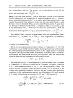
need to use a probability distribution. Figure S11.1 contrasts two processes with different
arrival distributions. The units arriving are shown as people, but they could be jobs arriving
at a machine, trucks needing servicing, or any other uncertain event. The top example shows
low variation in arrival time where customers arrive in a relatively predictable manner. The
bottom example has the same average number of customer arriving but this time they arrive
unpredictably with sometimes long gaps between arrivals and at other times two or three
customers arriving close together. Of course, we could do a similar analysis to describe processing times. Again, some would have low variation, some higher variation and others be
somewhere in between.
In Figure S11.1 high arrival variation has a distribution with a wider spread (called
‘dispersion’) than the distribution describing lower variability. Statistically the usual measure
for indicating the spread of a distribution is its standard deviation, σ. But variation does not
only depend on standard deviation. For example, a distribution of arrival times may have
a standard deviation of 2 minutes. This could indicate very little variation when the average
arrival time is 60 minutes. But it would mean a very high degree of variation when the


M11B_SLAC0460_06_SE_C11B.QXD

10/20/09

9:43

Page 335

Supplement to Chapter 11 Analytical queuing models

Figure S11.1 Low and high arrival variation

average arrival time is 3 minutes. Therefore to normalize standard deviation, it is divided
by the mean of its distribution. This measure is called the coefficient of variation of the

distribution. So,
ca = coefficient of variation of arrival times = σa /ta
ce = coefficient of variation of processing times = σe /te

Incorporating Little’s law
In Chapter 4 we discussed on of the fundamental laws of processes that describes the relationship between the cycle time of a process (how often something emerges from the process),
the working in progress in the process and the throughput time of the process (the total time
it takes for an item to move through the whole process including waiting time). It was called
Little’s law and it was denoted by the following simple relationship.
Work-in-progress = cycle time × throughput time
Or,
WIP = C × T
We can make use of Little’s law to help understand queuing behaviour. Consider the queue
in front of a station.
Work-in-progress in the queue = the arrival rate at the queue (equivalent to cycle time)
× waiting time in the queue (equivalent to throughput
time)
WIPq = ra × Wq
and
Waiting time in the whole system = the waiting time in the queue + the average process
time at the station
W = Wq + te
We will use this relationship later to investigate queuing behaviour.

335


M11B_SLAC0460_06_SE_C11B.QXD

336

10/20/09

9:43

Page 336

Part Three Planning and control

Types of queuing system
Conventionally queuing systems are characterized by four parameters.
A – the distribution of arrival times (or more properly interarrival times, the elapsed
times between arrivals)
B – the distribution of process times
m – the number of servers at each station
b – the maximum number of items allowed in the system.
The most common distributions used to describe A or B are either
(a) the exponential (or Markovian) distribution denoted by M; or
(b) the general (for example normal) distribution denoted by G.
So, for example, an M/G/1/5 queuing system would indicate a system with exponentially
distributed arrivals, process times described by a general distribution such as a normal distribution, with one server and a maximum number of items allowed in the system of 5. This
type of notation is called Kendall’s notation.
Queuing theory can help us investigate any type of queuing system, but in order to
simplify the mathematics, we shall here deal only with the two most common situations.
Namely,
M/M/m queues

●

G/G/m queues

●

M/M/m – the exponential arrival and processing times with m servers and no maximum
limit to the queue.
G/G/m – general arrival and processing distributions with m servers and no limit to the
queue.

And first we will start by looking at the simple case when m = 1.

For M/M/1 queuing systems
The formulae for this type of system are as follows.
WIP =

u
1−u

Using Little’s law,
WIP = cycle time × throughput time
Throughput time = WIP / cycle time
Then,
Throughput time =

u
1
t
× = e
1 − u ra 1 − u

and since, throughput time in the queue = total throughput time − average processing time,

Wq = W − te
=

te
− te
1−u

=

te − te(1 − u) te − te − ute
=
1−u
1−u

=

u
te
(1 − u)


M11B_SLAC0460_06_SE_C11B.QXD

10/20/09

9:43

Page 337

Supplement to Chapter 11 Analytical queuing models

again, using Little’s law
WIPq = ra × Wq =

u
tera
(1 − u)

and since
u=

ra
= rate
re

ra =

u
te

then,
WIPq =
=

u
u
× te ×
(1 − u)
te
u2

(1 − u)

For M/M/m systems
When there are m servers at a station the formula for waiting time in the queue (and therefore all other formulae) needs to be modified. Again, we will not derive these formulae but
just state them.
Wq =

u 2(m+1)−1
te
m(1 − u)

From which the other formulae can be derived as before.

For G/G/1 systems
The assumption of exponential arrival and processing times is convenient as far as the
mathematical derivation of various formulae are concerned. However, in practice, process
times in particular are rarely truly exponential. This is why it is important to have some idea
of how a G/G/1 and G/G/m queue behaves. However, exact mathematical relationships are
not possible with such distributions. Therefore some kind of approximation is needed. The
one here is in common use, and although it is not always accurate, it is for practical purposes.
For G/G/1 systems the formula for waiting time in the queue is as follows.
Wq =

VUT formula

A ca2 + ce2 D A u D
t
C 2 F C (1 − u)F e

There are two points to make about this equation. The first is that it is exactly the same as the

equivalent equation for an M/M/1 system but with a factor to take account of the variability
of the arrival and process times. The second is that this formula is sometimes known as the
VUT formula because it describes the waiting time in a queue as a function of:
V – the variability in the queuing system
U – the utilization of the queuing system (that is demand versus capacity), and
T – the processing times at the station.
In other words, we can reach the intuitive conclusion that queuing time will increase as
variability, utilization or processing time increases.

337


M11B_SLAC0460_06_SE_C11B.QXD

338

10/20/09

9:43

Page 338

Part Three Planning and control

For G/G/m systems
The same modification applies to queuing systems using general equations and m servers.
The formula for waiting time in the queue is now as follows.
Wq =

A ca2 + ce2 D A u 2(m+1)−1 D

t
C 2 F C m(1 − u)F e

Worked example 1
‘I can’t understand it. We have worked out our capacity figures and I am sure that one
member of staff should be able to cope with the demand. We know that customers arrive
at a rate of around 6 per hour and we also know that any trained member of staff can
process them at a rate of 8 per hour. So why is the queue so large and the wait so long?
Have at look at what is going on there please.’
Sarah knew that it was probably the variation, both in customers arriving and in how
long it took each of them to be processed, that was causing the problem. Over a two-day
period when she was told that demand was more or less normal, she timed the exact
arrival times and processing times of every customer. Her results were as follows.
The coefficient of variation, ca of customer arrivals = 1
The coefficient of variation, ce of processing time = 3.5
The average arrival rate of customers, ra
= 6 per hour
therefore, the average inter-arrival time
= 10 minutes
The average processing rate, re
= 8 per hour
therefore, the average processing time
= 7.5 minutes
Therefore the utilization of the single server, u
= 6/8 = 0.75
Using the waiting time formula for a G/G/1 queuing system
Wq =

A 1 + 12.25 D A 0.75 D
7.5

C
F C 1 − 0.75 F
2

= 6.625 × 3 × 7.5 = 149.06 mins
= 2.48 hours
Also because,
WIPq = cycle time × throughput time
WIPq = 6 × 2.48 = 14.68
So, Sarah had found out that the average wait that customers could expect was 2.48 hours
and that there would be an average of 14.68 people in the queue.
‘Ok, so I see that it’s the very high variation in the processing time that is causing the queue
to build up. How about investing in a new computer system that would standardize
processing time to a greater degree? I have been talking with our technical people and
they reckon that, if we invested in a new system, we could cut the coefficient of variation
of processing time down to 1.5. What kind of a different would this make?’
Under these conditions with ce = 1.5
Wq =

A 1 + 2.25 D A 0.75 D
7.5
C
2 F C 1 − 0.75 F

= 1.625 × 3 × 7.5 = 36.56 mins
= 0.61 hour


M11B_SLAC0460_06_SE_C11B.QXD

10/20/09

9:43

Page 339

Supplement to Chapter 11 Analytical queuing models

Therefore,
WIPq = 6 × 0.61 = 3.66
In other words, reducing the variation of the process time has reduced average queuing
time from 2.48 hours down to 0.61 hour and has reduced the expected number of
people in the queue from 14.68 down to 3.66.

Worked example 2
A bank wishes to decide how many staff to schedule during its lunch period. During
this period customers arrive at a rate of 9 per hour and the enquiries that customers
have (such as opening new accounts, arranging loans, etc.) take on average 15 minutes
to deal with. The bank manager feels that four staff should be on duty during this period
but wants to make sure that the customers do not wait more than 3 minutes on average
before they are served. The manager has been told by his small daughter that the distributions that describe both arrival and processing times are likely to be exponential.
Therefore,
ra = 9 per hour, therefore
ta = 6.67 minutes
re = 4 per hour, therefore
te = 15 minutes
The proposed number of servers, m = 4
therefore, the utilization of the system, u = 9/(4 × 4) = 0.5625.
From the formula for waiting time for a M/M/m system,
Wq =

u 2(m+1)−1
te
m(1 − u)

Wq =

0.5625 10−1
× 0.25
4(1 − 0.5625)

=

0.56252.162
1.75

× 0.25

= 0.042 hour
= 2.52 minutes
Therefore the average waiting time with 4 servers would be 2.52 minutes, which is well
within the manager’s acceptable waiting tolerance.

339


M12_SLAC0460_06_SE_C12.QXD

10/20/09

Chapter

9:45

12

Page 340

Inventory planning
and control

Introduction

Key questions
➤ What is inventory?
➤ Why is inventory necessary?
➤ What are the disadvantages of
holding inventory?
➤ How much inventory should an
operation hold?
➤ When should an operation replenish
its inventory?
➤ How can inventory be controlled?

Operations managers often have an ambivalent attitude towards
inventories. On the one hand, they are costly, sometimes tying
up considerable amounts of working capital. They are also risky
because items held in stock could deteriorate, become obsolete
or just get lost, and, furthermore, they take up valuable space in
the operation. On the other hand, they provide some security in

an uncertain environment that one can deliver items in stock,
should customers demand them. This is the dilemma of inventory
management: in spite of the cost and the other disadvantages
associated with holding stocks, they do facilitate the smoothing
of supply and demand. In fact they only exist because supply
and demand are not exactly in harmony with each other
(see Fig. 12.1).

Figure 12.1 This chapter covers inventory planning and control

Check and improve your understanding of this chapter using self assessment
questions and a personalised study plan, audio and video downloads, and an
eBook – all at www.myomlab.com.


M12_SLAC0460_06_SE_C12.QXD

10/20/09

9:45

Page 341

Chapter 12

341

Inventory planning and control

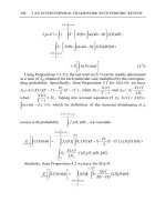
Operations in practice The UK’s National Blood Service1

1 Collection, which involves recruiting and retaining
blood donors, encouraging them to attend donor
sessions (at mobile or fixed locations) and transporting
the donated blood to their local blood centre.
2 Processing, which breaks blood down into its
constituent parts (red cells, platelets and plasma)
as well over twenty other blood-based ‘products’.
3 Distribution, which transports blood from blood
centres to hospitals in response to both routine and
emergency requests. Of the Service’s 200,000
deliveries a year, about 2,500 are emergency
deliveries.
Inventory accumulates at all three stages, and in
individual hospitals’ blood banks. Within the supply
chain, around 11.5 per cent of donated red blood cells
donated are lost. Much of this is due to losses in
processing, but around 5 per cent is not used because
it has ‘become unavailable’, mainly because it has been
stored for too long. Part of the Service’s inventory control
task is to keep this ‘time-expired’ loss to a minimum.
In fact, only small losses occur within the NBS, most
blood being lost when it is stored in hospital blood banks
that are outside its direct control. However, it does
attempt to provide advice and support to hospitals to
enable them to use blood efficiently.
Blood components and products need to be stored
under a variety of conditions, but will deteriorate
over time. This varies depending on the component;
platelets have a shelf life of only five days and demand

can fluctuate significantly. This makes stock control
particularly difficult. Even red blood cells that have a

Source: Alamy/Van Hilversum

No inventory manager likes to run out of stock. But for
blood services, such as the UK’s National Blood Service
(NBS) the consequences of running out of stock can
be particularly serious. Many people owe their lives to
transfusions that were made possible by the efficient
management of blood, stocked in a supply network
that stretches from donation centres through to hospital
blood banks. The NBS supply chain has three main
stages:

shelf life of 35 days may not be acceptable to hospitals
if they are close to their ‘use-by date’. Stock accuracy
is crucial. Giving a patient the wrong type of blood can
be fatal.
At a local level demand can be affected significantly
by accidents. One serious accident involving a cyclist
used 750 units of blood, which completely exhausted the
available supply (miraculously, he survived). Large-scale
accidents usually generate a surge of offers from donors
wishing to make immediate donations. There is also a
more predictable seasonality to the donating of blood,
however, with a low period during the summer vacation.
Yet there is always an unavoidable tension between
maintaining sufficient stocks to provide a very high level
of supply dependability to hospitals and minimizing

wastage. Unless blood stocks are controlled carefully,
they can easily go past the ‘use-by date’ and be wasted.
But avoiding outdated blood products is not the only
inventory objective at NBS. It also measures the
percentage of requests that it was able to meet in full,
the percentage emergency requests delivered within
two hours, the percentage of units banked to donors
bled, the number of new donors enrolled, and the
number of donors waiting longer than 30 minutes before
they are able to donate. The traceability of donated blood
is also increasingly important. Should any problems with
a blood product arise, its source can be traced back to
the original donor.


M12_SLAC0460_06_SE_C12.QXD

342

10/20/09

9:45

Page 342

Part Three Planning and control

What is inventory?
Inventory

Inventory, or ‘stock’ as it is more commonly called in some countries, is defined here as
the stored accumulation of material resources in a transformation system. Sometimes the term
‘inventory’ is also used to describe any capital-transforming resource, such as rooms in a
hotel, or cars in a vehicle-hire firm, but we will not use that definition here. Usually the term
refers only to transformed resources. So a manufacturing company will hold stocks of materials,
a tax office will hold stocks of information, and a theme park will hold stocks of customers.
Note that when it is customers who are being processed we normally refer to the ‘stocks’ of
them as ‘queues’. This chapter will deal particularly with inventories of materials.

Revisiting operations objectives; the roles of inventory
Most of us are accustomed to keeping inventory for use in our personal lives, but often we
don’t think about it. For example, most families have some stocks of food and drinks, so
that they don’t have to go out to the shops before every meal. Holding a variety of food
ingredients in stock in the kitchen cupboard or freezer gives us the ability to respond quickly
(with speed) in preparing a meal whenever unexpected guests arrive. It also allows us the
flexibility to choose a range of menu options without having to go to the time and trouble
of purchasing further ingredients. We may purchase some items because we have found
something of exceptional quality, but intend to save it for a special occasion. Many people
buy multiple packs to achieve lower costs for a wide range of goods. In general, our inventory
planning protects us from critical stock-outs; so this approach gives a level of dependability
of supplies.
It is, however, entirely possible to manage our inventory planning differently. For example,
some people (students?) are short of available cash and/or space, and so cannot ‘invest’ in
large inventories of goods. They may shop locally for much smaller quantities. They forfeit
the cost benefits of bulk-buying, but do not have to transport heavy or bulky supplies.
They also reduce the risk of forgetting an item in the cupboard and letting it go out of date.
Essentially, they purchase against specific known requirements (the next meal). However, they
may find that the local shop is temporarily out of stock of a particular item, forcing them,
for example, to drink coffee without their usual milk. How we control our own supplies
is therefore a matter of choice which can affect their quality (e.g. freshness), availability or

speed of response, dependability of supply, flexibility of choice, and cost. It is the same for
most organizations. Significant levels of inventory can be held for a range of sensible and
pragmatic reasons but it must also be tightly controlled for other equally good reasons.

Why is inventory necessary?
No matter what is being stored as inventory, or where it is positioned in the operation, it
will be there because there is a difference in the timing or rate of supply and demand. If
the supply of any item occurred exactly when it was demanded, the item would never be
stored. A common analogy is the water tank shown in Figure 12.2. If, over time, the rate of
supply of water to the tank differs from the rate at which it is demanded, a tank of water
(inventory) will be needed if supply is to be maintained. When the rate of supply exceeds the
rate of demand, inventory increases; when the rate of demand exceeds the rate of supply,
inventory decreases. So if an operation can match supply and demand rates, it will also
succeed in reducing its inventory levels.


M12_SLAC0460_06_SE_C12.QXD

10/20/09

9:45

Page 343

Chapter 12

Inventory planning and control

Figure 12.2 Inventory is created to compensate for the differences in timing between supply
and demand

Types of inventory
The various reasons for an imbalance between the rates of supply and demand at different points in any operation lead to the different types of inventory. There are five of these:
buffer inventory, cycle inventory, de-coupling inventory, anticipation inventory and pipeline
inventory.
Buffer inventory
Buffer inventory
Safety inventory

Buffer inventory is also called safety inventory. Its purpose is to compensate for the
unexpected fluctuations in supply and demand. For example, a retail operation can never
forecast demand perfectly, even when it has a good idea of the most likely demand level.
It will order goods from its suppliers such that there is always a certain amount of most
items in stock. This minimum level of inventory is there to cover against the possibility
that demand will be greater than expected during the time taken to deliver the goods. This
is buffer, or safety inventory. It can also compensate for the uncertainties in the process of
the supply of goods into the store, perhaps because of the unreliability of certain suppliers
or transport firms.
Cycle inventory

Cycle inventory

Cycle inventory occurs because one or more stages in the process cannot supply all the
items it produces simultaneously. For example, suppose a baker makes three types of bread,
each of which is equally popular with its customers. Because of the nature of the mixing and
baking process, only one kind of bread can be produced at any time. The baker would have
to produce each type of bread in batches (batch processes were described in Chapter 4)
as shown in Figure 12.3. The batches must be large enough to satisfy the demand for each
kind of bread between the times when each batch is ready for sale. So even when demand
is steady and predictable, there will always be some inventory to compensate for the intermittent supply of each type of bread. Cycle inventory only results from the need to produce

343


M12_SLAC0460_06_SE_C12.QXD

344

10/20/09

9:45

Page 344

Part Three Planning and control

Figure 12.3 Cycle inventory in a bakery

products in batches, and the amount of it depends on volume decisions which are described
in a later section of this chapter.
De-coupling Inventory

De-coupling inventory

Wherever an operation is designed to use a process layout (introduced in Chapter 7), the
transformed resources move intermittently between specialized areas or departments that
comprise similar operations. Each of these areas can be scheduled to work relatively independently in order to maximize the local utilization and efficiency of the equipment and
staff. As a result, each batch of work-in-progress inventory joins a queue, awaiting its turn
in the schedule for the next processing stage. This also allows each operation to be set to
the optimum processing speed (cycle time), regardless of the speed of the steps before and

after. Thus de-coupling inventory creates the opportunity for independent scheduling and
processing speeds between process stages.
Anticipation inventory

Anticipation inventory

In Chapter 11 we saw how anticipation inventory can be used to cope with seasonal demand.
Again, it was used to compensate for differences in the timing of supply and demand. Rather
than trying to make the product (such as chocolate) only when it was needed, it was produced throughout the year ahead of demand and put into inventory until it was needed.
Anticipation inventory is most commonly used when demand fluctuations are large but
relatively predictable. It might also be used when supply variations are significant, such as in
the canning or freezing of seasonal foods.
Pipeline inventory

Pipeline inventory

Pipeline inventory exists because material cannot be transported instantaneously between
the point of supply and the point of demand. If a retail store orders a consignment of items
from one of its suppliers, the supplier will allocate the stock to the retail store in its own
warehouse, pack it, load it onto its truck, transport it to its destination, and unload it into
the retailer’s inventory. From the time that stock is allocated (and therefore it is unavailable to any other customer) to the time it becomes available for the retail store, it is pipeline
inventory. Pipeline inventory also exists within processes where the layout is geographically
spread out. For example, a large European manufacturer of specialized steel regularly moves
cargoes of part-finished materials between its two mills in the UK and Scandinavia using
a dedicated vessel that shuttles between the two countries every week. All the thousands of
tonnes of material in transit are pipeline inventory.


M12_SLAC0460_06_SE_C12.QXD

10/20/09

9:45

Page 345

Chapter 12

Inventory planning and control

Some disadvantages of holding inventory
Although inventory plays an important role in many operations performance, there are a
number of negative aspects of inventory.
●

●
●
●
●
●
●
●

Inventory ties up money, in the form of working capital, which is therefore unavailable for
other uses, such as reducing borrowings or making investment in productive fixed assets
(we shall expand on the idea of working capital later).
Inventory incurs storage costs (leasing space, maintaining appropriate conditions, etc.).
Inventory may become obsolete as alternatives become available.
Inventory can be damaged, or deteriorate.
Inventory could be lost, or be expensive to retrieve, as it gets hidden amongst other inventory.

Inventory might be hazardous to store (for example flammable solvents, explosives,
chemicals and drugs), requiring special facilities and systems for safe handling.
Inventory uses space that could be used to add value.
Inventory involves administrative and insurance costs.

The position of inventory

Raw materials inventory
Components inventory
Work-in-progress
Finished goods inventory
Multi-echelon inventory

Not only are there several reasons for supply–demand imbalance, there could also be several
points where such imbalance exists between different stages in the operation. Figure 12.4
illustrates different levels of complexity of inventory relationships within an operation.
Perhaps the simplest level is the single-stage inventory system, such as a retail store, which
will have only one stock of goods to manage. An automotive parts distribution operation
will have a central depot and various local distribution points which contain inventories. In
many manufacturers of standard items, there are three types of inventory. The raw material
and components inventories (sometimes called input inventories) receive goods from the
operation’s suppliers; the raw materials and components work their way through the various
stages of the production process but spend considerable amounts of time as work-in-progress
(or work-in-process) (WIP) before finally reaching the finished goods inventory.
A development of this last system is the multi-echelon inventory system. This maps
the relationship of inventories between the various operations within a supply network
(see Chapter 6). In Figure 12.4(d) there are five interconnected sets of inventory systems. The
second-tier supplier’s (yarn producer’s) inventories will feed the first-tier supplier’s (cloth
producer’s) inventories, who will in turn supply the main operation. The products are distributed to local warehouses from where they are shipped to the final customers. We will
discuss the behaviour and management of such multi-echelon systems in the next chapter.

Day-to-day inventory decisions
At each point in the inventory system, operations managers need to manage the day-to-day
tasks of running the system. Orders will be received from internal or external customers;
these will be dispatched and demand will gradually deplete the inventory. Orders will need
to be placed for replenishment of the stocks; deliveries will arrive and require storing. In
managing the system, operations managers are involved in three major types of decision:
●
●
●

How much to order. Every time a replenishment order is placed, how big should it be
(sometimes called the volume decision)?
When to order. At what point in time, or at what level of stock, should the replenishment
order be placed (sometimes called the timing decision)?
How to control the system. What procedures and routines should be installed to help make
these decisions? Should different priorities be allocated to different stock items? How
should stock information be stored?

345


M12_SLAC0460_06_SE_C12.QXD

346

10/20/09

9:45

Page 346

Part Three Planning and control

Figure 12.4 (a) Single-stage, (b) two-stage, (c) multi-stage and (d) multi-echelon inventory systems

The volume decision – how much to order
To illustrate this decision, consider again the example of the food and drinks we keep at
our home. In managing this inventory we implicitly make decisions on order quantity,
which is how much to purchase at one time. In making this decision we are balancing two
sets of costs: the costs associated with going out to purchase the food items and the costs
associated with holding the stocks. The option of holding very little or no inventory of food
and purchasing each item only when it is needed has the advantage that it requires little
money since purchases are made only when needed. However, it would involve purchasing provisions several times a day, which is inconvenient. At the very opposite extreme,
making one journey to the local superstore every few months and purchasing all the provisions we would need until our next visit reduces the time and costs incurred in making the
purchase but requires a very large amount of money each time the trip is made – money


M12_SLAC0460_06_SE_C12.QXD

10/20/09

9:45

Page 347

Chapter 12

Inventory planning and control

which could otherwise be in the bank and earning interest. We might also have to invest in
extra cupboard units and a very large freezer. Somewhere between these extremes there
will lie an ordering strategy which will minimize the total costs and effort involved in the
purchase of food.
Inventory costs

The same principles apply in commercial order-quantity decisions as in the domestic situation.
In making a decision on how much to purchase, operations managers must try to identify
the costs which will be affected by their decision. Several types of costs are directly associated
with order size.
1 Cost of placing the order. Every time that an order is placed to replenish stock, a number
of transactions are needed which incur costs to the company. These include the clerical
tasks of preparing the order and all the documentation associated with it, arranging for
the delivery to be made, arranging to pay the supplier for the delivery, and the general
costs of keeping all the information which allows us to do this. Also, if we are placing an
‘internal order’ on part of our own operation, there are still likely to be the same types
of transaction concerned with internal administration. In addition, there could also be
a ‘changeover’ cost incurred by the part of the operation which is to supply the items,
caused by the need to change from producing one type of item to another.
2 Price discount costs. In many industries suppliers offer discounts on the normal purchase
price for large quantities; alternatively they might impose extra costs for small orders.
3 Stock-out costs. If we misjudge the order-quantity decision and our inventory runs out
of stock, there will be costs to us incurred by failing to supply our customers. If the
customers are external, they may take their business elsewhere; if internal, stock-outs
could lead to idle time at the next process, inefficiencies and, eventually, again, dissatisfied
external customers.
4 Working capital costs. Soon after we receive a replenishment order, the supplier will demand
payment for their goods. Eventually, when (or after) we supply our own customers, we
in turn will receive payment. However, there will probably be a lag between paying our
suppliers and receiving payment from our customers. During this time we will have to

fund the costs of inventory. This is called the working capital of inventory. The costs
associated with it are the interest we pay the bank for borrowing it, or the opportunity
costs of not investing it elsewhere.
5 Storage costs. These are the costs associated with physically storing the goods. Renting,
heating and lighting the warehouse, as well as insuring the inventory, can be expensive,
especially when special conditions are required such as low temperature or high security.
6 Obsolescence costs. When we order large quantities, this usually results in stocked items
spending a long time stored in inventory. Then there is a risk that the items might either
become obsolete (in the case of a change in fashion, for example) or deteriorate with age
(in the case of most foodstuffs, for example).
7 Operating inefficiency costs. According to lean synchronization philosophies, high inventory
levels prevent us seeing the full extent of problems within the operation. This argument is
fully explored in Chapter 15.

Consignment stock

There are two points to be made about this list of costs. The first is that some of the
costs will decrease as order size is increased; the first three costs are like this, whereas the
other costs generally increase as order size is increased. The second point is that it may not
be the same organization that incurs the costs. For example, sometimes suppliers agree to
hold consignment stock. This means that they deliver large quantities of inventory to their
customers to store but will only charge for the goods as and when they are used. In the meantime they remain the supplier’s property so do not have to be financed by the customer, who
does, however, provide storage facilities.

347


M12_SLAC0460_06_SE_C12.QXD

348

10/20/09

9:45

Page 348

Part Three Planning and control

Short case
Croft Port
Not all inventory is purely a source of cost. Some
industries rely on it to add value. Oporto, a Portuguese
city famous for port wine is awash with inventory. While
wines in the style of port are produced around the world
in several countries, including Australia and South Africa,
only the product from Portugal may be labelled as port.
One of the famous port brands is Croft Port which was
founded in 1678. It owns one of the best wine-growing
estates in the Douro valley, Quinta da Roêda. When
the grapes have been picked they are crushed at the
wineries (in the Douro valley). They used to be crushed
by treading by foot with a row of people holding on to
each other and walking back and forth across the granite
‘baths’ filled with the grapes. Now mechanical methods
are used. As the grapes are squashed fermentation
begins as the natural sugars in the juice are converted
into alcohol by micro-organisms (yeast) in the grapes.

The grape skins are retained during crushing to ensure

their colour and tannins are released into the wine. After
a while the skins are allowed to float to the surface and
the fermenting juice is drawn from underneath. It is then
mixed with a neutral grape spirit (fortification) to raise
the strength of the wine and also stop fermentation in
order to preserve some of the natural grape sugars in
the finished product. The wine is then stored and aged
in barrels in the cool dark caves (cellars) in Vila Nova de
Gaia to allow the wine to mellow and develop its flavours
before being bottled. There are essentially two styles of
port, wood-aged and bottle-aged. Most port wines are
wood-aged in oak vats or casks for five or six years for
full-bodied wines or for 10–20 years for tawny ports.
They are then bottled and ready to drink. The main type
of bottle-aged port is vintage port, the best and rarest of
all ports. This is made up of a selection of the very best
grapes from the harvest of exceptional years. Although
this port is only stored in the oak barrels for two years
it is then allowed to mature and age in the bottles for
many years, often decades.

Inventory profiles

An inventory profile is a visual representation of the inventory level over time. Figure 12.5
shows a simplified inventory profile for one particular stock item in a retail operation. Every
time an order is placed, Q items are ordered. The replenishment order arrives in one batch
instantaneously. Demand for the item is then steady and perfectly predictable at a rate of
D units per month. When demand has depleted the stock of the items entirely, another order
of Q items instantaneously arrives, and so on. Under these circumstances:
Q

(because the two shaded areas in Fig. 12.5 are equal)
2
Q
The time interval between deliveries =
D
D
The frequency of deliveries = the reciprocal of the time interval =
Q
The average inventory =

Figure 12.5 Inventory profiles chart the variation in inventory level


M12_SLAC0460_06_SE_C12.QXD

10/20/09

9:45

Page 349

Chapter 12

Inventory planning and control

Figure 12.6 Two alternative inventory plans with different order quantities (Q)

The economic order quantity (EOQ) formula
Economic order quantity

The most common approach to deciding how much of any particular item to order when
stock needs replenishing is called the economic order quantity (EOQ) approach. This approach
attempts to find the best balance between the advantages and disadvantages of holding stock.
For example, Figure 12.6 shows two alternative order-quantity policies for an item. Plan A,
represented by the unbroken line, involves ordering in quantities of 400 at a time. Demand
in this case is running at 1,000 units per year. Plan B, represented by the dotted line, uses
smaller but more frequent replenishment orders. This time only 100 are ordered at a time,
with orders being placed four times as often. However, the average inventory for plan B is
one-quarter of that for plan A.
To find out whether either of these plans, or some other plan, minimizes the total cost
of stocking the item, we need some further information, namely the total cost of holding one
unit in stock for a period of time (Ch) and the total costs of placing an order (Co). Generally,
holding costs are taken into account by including:
●
●
●

working capital costs
storage costs
obsolescence risk costs.

Order costs are calculated by taking into account:
●
●

cost of placing the order (including transportation of items from suppliers if relevant);
price discount costs.

In this case the cost of holding stocks is calculated at £1 per item per year and the cost of
placing an order is calculated at £20 per order.

We can now calculate total holding costs and ordering costs for any particular ordering
plan as follows:
Holding costs = holding cost/unit × average inventory
= Ch ×

Q
2

Ordering costs = ordering cost × number of orders per period
= Co ×
So, total cost, Ct =

D
Q

ChQ CoD
+
2
Q

349


M12_SLAC0460_06_SE_C12.QXD

350

10/20/09

9:45

Page 350

Part Three Planning and control
Table 12.1 Costs of adoption of plans with different order quantities
Demand (D) = 1,000 units per year
Order costs (Co ) = £20 per order
Order quantity
(Q)
50
100
150
200
250
300
350
400

Holding costs
(0.5Q × Ch )

Holding costs (Ch ) = £1 per item per year
+

25
50
75
100
125
150

175
200

Order costs
((D/Q) × Co )
20 × 20 = 400
10 × 20 = 200
6.7 × 20 = 134
5 × 20 = 100
4 × 20 = 80
3.3 × 20 = 66
2.9 × 20 = 58
2.5 × 20 = 50

=

Total costs
425
250
209
200*
205
216
233
250

*Minimum total cost.

We can now calculate the costs of adopting plans with different order quantities. These are
illustrated in Table 12.1. As we would expect with low values of Q, holding costs are low but

the costs of placing orders are high because orders have to be placed very frequently. As Q
increases, the holding costs increase but the costs of placing orders decrease. Initially the
decrease in ordering costs is greater than the increase in holding costs and the total cost falls.
After a point, however, the decrease in ordering costs slows, whereas the increase in holding
costs remains constant and the total cost starts to increase. In this case the order quantity, Q,
which minimizes the sum of holding and order costs, is 200. This ‘optimum’ order quantity
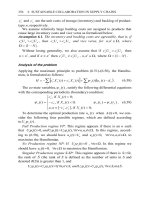
is called the economic order quantity (EOQ). This is illustrated graphically in Figure 12.7.

Figure 12.7 Graphical representation of the economic order quantity


M12_SLAC0460_06_SE_C12.QXD

10/20/09

9:45

Page 351

Chapter 12

Inventory planning and control

351

A more elegant method of finding the EOQ is to derive its general expression. This can be
done using simple differential calculus as follows. From before:
Total cost = holding cost + order cost
Ct =

ChQ CoD
+
2
Q

The rate of change of total cost is given by the first differential of Ct with respect to Q:
dCt Ch CoD
=
− 2
dQ
2
Q
The lowest cost will occur when dCt /dQ = 0, that is:
0=

Ch CoD
−
2
Qo2

where Qo = the EOQ. Rearranging this expression gives:
Qo = EOQ =

2CoD
Ch

When using the EOQ:
Time between orders =
Order frequency =

EOQ
D

D
per period
EOQ

Sensitivity of the EOQ

Examination of the graphical representation of the total cost curve in Figure 12.7 shows
that, although there is a single value of Q which minimizes total costs, any relatively small
deviation from the EOQ will not increase total costs significantly. In other words, costs will
be near-optimum provided a value of Q which is reasonably close to the EOQ is chosen. Put
another way, small errors in estimating either holding costs or order costs will not result in a
significant deviation from the EOQ. This is a particularly convenient phenomenon because,
in practice, both holding and order costs are not easy to estimate accurately.

Worked example
A building materials supplier obtains its bagged cement from a single supplier. Demand
is reasonably constant throughout the year, and last year the company sold 2,000 tonnes
of this product. It estimates the costs of placing an order at around £25 each time an
order is placed, and calculates that the annual cost of holding inventory is 20 per cent of
purchase cost. The company purchases the cement at £60 per tonne. How much should
the company order at a time?
EOQ for cement =

2CoD
Ch

=

2 × 25 × 2,000
0.2 × 60

=

100,000
12

= 91.287 tonnes

➔


M12_SLAC0460_06_SE_C12.QXD

352

10/20/09

9:45

Page 352

Part Three Planning and control

After calculating the EOQ the operations manager feels that placing an order for
91.287 tonnes exactly seems somewhat over-precise. Why not order a convenient
100 tonnes?
Total cost of ordering plan for Q = 91.287:

=

ChQ Co D
+
2
Q

=

(0.2 × 60) × 91.287 25 × 2,000
+
2
91.287

= £1,095.454
Total cost of ordering plan for Q = 100:
=

(0.2 × 60) × 100 25 × 2,000
+
2
100

= £1,100
The extra cost of ordering 100 tonnes at a time is £1,100 − £1,095.45 = £4.55. The
operations manager therefore should feel confident in using the more convenient order
quantity.

Gradual replacement – the economic batch quantity
(EBQ) model

Although the simple inventory profile shown in Figure 12.5 made some simplifying assumptions, it is broadly applicable in most situations where each complete replacement order
arrives at one point in time. In many cases, however, replenishment occurs over a time
period rather than in one lot. A typical example of this is where an internal order is placed
for a batch of parts to be produced on a machine. The machine will start to produce the
parts and ship them in a more or less continuous stream into inventory, but at the same time
demand is continuing to remove parts from the inventory. Provided the rate at which parts
are being made and put into the inventory (P) is higher than the rate at which demand is
depleting the inventory (D), then the size of the inventory will increase. After the batch has
been completed the machine will be reset (to produce some other part), and demand will
continue to deplete the inventory level until production of the next batch begins. The resulting profile is shown in Figure 12.8. Such a profile is typical for cycle inventories supplied by

Figure 12.8 Inventory profile for gradual replacement of inventory


M12_SLAC0460_06_SE_C12.QXD

10/20/09

9:45

Page 353

Chapter 12

Economic batch quantity

Inventory planning and control

353

batch processes, where items are produced internally and intermittently. For this reason the
minimum-cost batch quantity for this profile is called the economic batch quantity (EBQ).
It is also sometimes known as the economic manufacturing quantity (EMQ), or the production order quantity (POQ). It is derived as follows:
Maximum stock level = M
Slope of inventory build-up = P − D
Also, as is clear from Figure 12.8:
Slope of inventory build-up = M ÷
=

Q
P

MP
Q

So,
MP
=P−D
Q
M=
Average inventory level =
=

Q(P − D)
P
M
2
Q(P − D)
2P

As before:
Total cost = holding cost + order cost
Ct =

ChQ(P − D) CoD
+
2P
Q

dCt Ch(P − D) CoD
=
− 2
dQ
2P
Q
Again, equating to zero and solving Q gives the minimum-cost order quantity EBQ:
EBQ =

2CoD
Ch(1 − (D/P))

Worked example
The manager of a bottle-filling plant which bottles soft drinks needs to decide how long
a ‘run’ of each type of drink to process. Demand for each type of drink is reasonably
constant at 80,000 per month (a month has 160 production hours). The bottling lines fill
at a rate of 3,000 bottles per hour, but take an hour to clean and reset between different
drinks. The cost (of labour and lost production capacity) of each of these changeovers
has been calculated at £100 per hour. Stock-holding costs are counted at £0.1 per bottle
per month.

➔


M12_SLAC0460_06_SE_C12.QXD

354

10/20/09

9:45

Page 354

Part Three Planning and control

D = 80,000 per month
= 500 per hour
2CoD
Ch(1 − (D/P))

EBQ =

2 × 100 × 80,000
0.1(1 − (500/3,000))

=

EBQ = 13,856
The staff who operate the lines have devised a method of reducing the changeover time
from 1 hour to 30 minutes. How would that change the EBQ?

New Co = £50
New EBQ =

2 × 50 × 80,000
0.1(1 − (500/3,000))

= 9,798

Critical commentary
The approach to determining order quantity which involves optimizing costs of holding stock
against costs of ordering stock, typified by the EOQ and EBQ models, has always been
subject to criticisms. Originally these concerned the validity of some of the assumptions
of the model; more recently they have involved the underlying rationale of the approach
itself. The criticisms fall into four broad categories, all of which we shall examine further:
●

The assumptions included in the EOQ models are simplistic.
The real costs of stock in operations are not as assumed in EOQ models.
● The models are really descriptive, and should not be used as prescriptive devices.
● Cost minimization is not an appropriate objective for inventory management.
●

Responding to the criticisms of EOQ
In order to keep EOQ-type models relatively straightforward, it was necessary to make
assumptions. These concerned such things as the stability of demand, the existence of a fixed
and identifiable ordering cost, that the cost of stock holding can be expressed by a linear
function, shortage costs which were identifiable, and so on. While these assumptions are rarely
strictly true, most of them can approximate to reality. Furthermore, the shape of the total cost
curve has a relatively flat optimum point which means that small errors will not significantly
affect the total cost of a near-optimum order quantity. However, at times the assumptions

do pose severe limitations to the models. For example, the assumption of steady demand
(or even demand which conforms to some known probability distribution) is untrue for a
wide range of the operation’s inventory problems. For example, a bookseller might be very
happy to adopt an EOQ-type ordering policy for some of its most regular and stable products such as dictionaries and popular reference books. However, the demand patterns for
many other books could be highly erratic, dependent on critics’ reviews and word-of-mouth
recommendations. In such circumstances it is simply inappropriate to use EOQ models.
Cost of stock

Other questions surround some of the assumptions made concerning the nature of stockrelated costs. For example, placing an order with a supplier as part of a regular and multi-item
order might be relatively inexpensive, whereas asking for a special one-off delivery of an item


M12_SLAC0460_06_SE_C12.QXD

10/20/09

9:45

Page 355

Chapter 12

Inventory planning and control

could prove far more costly. Similarly with stock-holding costs – although many companies
make a standard percentage charge on the purchase price of stock items, this might not be
appropriate over a wide range of stock-holding levels. The marginal costs of increasing stockholding levels might be merely the cost of the working capital involved. On the other hand,
it might necessitate the construction or lease of a whole new stock-holding facility such as a
warehouse. Operations managers using an EOQ-type approach must check that the decisions
implied by the use of the formulae do not exceed the boundaries within which the cost

assumptions apply. In Chapter 15 we explore the just-in-time approach which sees inventory
as being largely negative. However, it is useful at this stage to examine the effect on an EOQ
approach of regarding inventory as being more costly than previously believed. Increasing
the slope of the holding cost line increases the level of total costs of any order quantity, but
more significantly, shifts the minimum cost point substantially to the left, in favour of a lower
economic order quantity. In other words, the less willing an operation is to hold stock on the
grounds of cost, the more it should move towards smaller, more frequent ordering.
Using EOQ models as prescriptions

Perhaps the most fundamental criticism of the EOQ approach again comes from the
Japanese-inspired ‘lean’ and JIT philosophies. The EOQ tries to optimize order decisions.
Implicitly the costs involved are taken as fixed, in the sense that the task of operations
managers is to find out what are the true costs rather than to change them in any way. EOQ
is essentially a reactive approach. Some critics would argue that it fails to ask the right
question. Rather than asking the EOQ question of ‘What is the optimum order quantity?’,
operations managers should really be asking, ‘How can I change the operation in some way
so as to reduce the overall level of inventory I need to hold?’ The EOQ approach may be a
reasonable description of stock-holding costs but should not necessarily be taken as a strict
prescription over what decisions to take. For example, many organizations have made considerable efforts to reduce the effective cost of placing an order. Often they have done this
by working to reduce changeover times on machines. This means that less time is taken
changing over from one product to the other, and therefore less operating capacity is lost,
which in turn reduces the cost of the changeover. Under these circumstances, the order
cost curve in the EOQ formula reduces and, in turn, reduces the effective economic order
quantity. Figure 12.9 shows the EOQ formula represented graphically with increased holding costs (see the previous discussion) and reduced order costs. The net effect of this is to
significantly reduce the value of the EOQ.
Should the cost of inventory be minimized?

Many organizations (such as supermarkets and wholesalers) make most of their revenue
and profits simply by holding and supplying inventory. Because their main investment is
in the inventory it is critical that they make a good return on this capital, by ensuring that

it has the highest possible ‘stock turn’ (defined later in this chapter) and/or gross profit
margin. Alternatively, they may also be concerned to maximize the use of space by seeking
to maximize the profit earned per square metre. The EOQ model does not address these
objectives. Similarly for products that deteriorate or go out of fashion, the EOQ model can
result in excess inventory of slower-moving items. In fact, the EOQ model is rarely used in
such organizations, and there is more likely to be a system of periodic review (described later)
for regular ordering of replenishment inventory. For example, a typical builders’ supply
merchant might carry around 50,000 different items of stock (SKUs – stock-keeping units).
However, most of these cluster into larger families of items such as paints, sanitaryware or
metal fixings. Single orders are placed at regular intervals for all the required replenishments
in the supplier’s range, and these are then delivered together at one time. For example,
if such deliveries were made weekly, then on average, the individual item order quantities
will be for only one week’s usage. Less popular items, or ones with erratic demand patterns,
can be individually ordered at the same time, or (when urgent) can be delivered the next
day by carrier.

355


M12_SLAC0460_06_SE_C12.QXD

9:45

Page 356

Part Three Planning and control

Figure 12.9 If the true costs of stock holding are taken into account, and if the cost of
ordering (or changeover) is reduced, the economic order quantity (EOQ) is much smaller

Short case
Howard Smith Paper Group2
The Howard Smith Paper Group operates the most
advanced warehousing operation within the European
paper merchanting sector, delivering over 120,000 tonnes
of paper annually. The function of a paper merchant is to
provide the link between the paper mills and the printers
or converters. This is illustrated in Figure 12.10. It is a
sales- and service-driven business, so the role of the
operation function is to deliver whatever the salesperson
has promised to the customer. Usually, this means
precisely the right product at the right time at the right
place and in the right quantity. The company’s operations
are divided into two areas, ‘logistics’ which combines
all warehousing and logistics tasks, and ‘supply side’
which includes inventory planning, purchasing and
merchandizing decisions. Its main stocks are held at
the national distribution centre, located in Northampton
in the middle part of the UK. This location was chosen
because it is at the centre of the company’s main
customer location and also because it has good access
to motorways. The key to any efficient merchanting
operation lies in its ability to do three things well.
First, it must efficiently store the desired volume of
required inventory. Second, it must have a ‘goods

Source: Howard Smith Paper Group

356

10/20/09

Dispatch activity at Howard Smith Paper Group

inward’ programme that sources the required volume
of desired inventory. Third, it must be able to fulfil
customer orders by ‘picking’ the desired goods fast
and accurately from its warehouse. The warehouse is
operational 24 hours per day, 5 days per week. A total
of 52 staff are employed in the warehouse, including
maintenance and cleaning staff. Skill sets are not an
issue, since all pickers are trained for all tasks. This
facilitates easier capacity management, since pickers
can be deployed where most urgently needed. Contract
labour is used on occasions, although this is less


M12_SLAC0460_06_SE_C12.QXD

10/20/09

9:45

Page 357

Chapter 12

Inventory planning and control

Figure 12.10 The role of the paper merchant

effective because the staff tend to be less motivated,
and have to learn the job.
At the heart of the company’s operations is a
warehouse known as a ‘dark warehouse’. All picking and
movement within the dark warehouse is fully automatic
and there is no need for any person to enter the high-bay
stores and picking area. The important difference with this
warehouse operation is that pallets are brought to the
pickers. Conventional paper merchants send pickers with
handling equipment into the warehouse aisles for stock.
A warehouse computer system (WCS) controls the whole
operation without the need for human input. It manages
pallet location and retrieval, robotic crane missions,

automatic conveyors, bar-code label production and
scanning, and all picking routines and priorities. It also
calculates operator activity and productivity measures,
as well as issuing documentation and planning
transportation schedules. The fact that all products are
identified by a unique bar code means that accuracy is
guaranteed. The unique user log-on ensures that any
picking errors can be traced back to the name of the
picker, to ensure further errors do not occur. The WCS
is linked to the company’s ERP system (we will deal with
ERP in Chapter 14), such that once the order has been
placed by a customer, computers manage the whole
process from order placement to order dispatch.

The timing decision – when to place an order

Re-order point

When we assumed that orders arrived instantaneously and demand was steady and predictable, the decision on when to place a replenishment order was self-evident. An order would be
placed as soon as the stock level reached zero. This would arrive instantaneously and prevent
any stock-out occurring. If replenishment orders do not arrive instantaneously, but have
a lag between the order being placed and it arriving in the inventory, we can calculate the
timing of a replacement order as shown in Figure 12.11. The lead time for an order to arrive
is in this case two weeks, so the re-order point (ROP) is the point at which stock will fall to
zero minus the order lead time. Alternatively, we can define the point in terms of the level

357