OReilly r for data science visualize model transform tidy and import data
Bạn đang xem bản rút gọn của tài liệu. Xem và tải ngay bản đầy đủ của tài liệu tại đây (32.31 MB, 520 trang )
R for Data
Science
IMPORT, TIDY, TRANSFORM, VISUALIZE, AND MODEL DATA
Hadley Wickham &
Garrett Grolemund
R for Data Science
Import, Tidy, Transform, Visualize,
and Model Data
Hadley Wickham and Garrett Grolemund
Beijing
Boston Farnham Sebastopol
Tokyo
R for Data Science
by Hadley Wickham and Garrett Grolemund
Copyright © 2017 Garrett Grolemund, Hadley Wickham. All rights reserved.
Printed in Canada.
Published by O’Reilly Media, Inc., 1005 Gravenstein Highway North, Sebastopol, CA
95472.
O’Reilly books may be purchased for educational, business, or sales promotional use.
Online editions are also available for most titles ( For more
information, contact our corporate/institutional sales department: 800-998-9938 or
Editors: Marie Beaugureau and
Mike Loukides
Production Editor: Nicholas Adams
Copyeditor: Kim Cofer
Proofreader: Charles Roumeliotis
December 2016:
Indexer: Wendy Catalano
Interior Designer: David Futato
Cover Designer: Karen Montgomery
Illustrator: Rebecca Demarest
First Edition
Revision History for the First Edition
2016-12-06:
First Release
See for release details.
The O’Reilly logo is a registered trademark of O’Reilly Media, Inc. R for Data Sci‐
ence, the cover image, and related trade dress are trademarks of O’Reilly Media, Inc.
While the publisher and the authors have used good faith efforts to ensure that the
information and instructions contained in this work are accurate, the publisher and
the authors disclaim all responsibility for errors or omissions, including without
limitation responsibility for damages resulting from the use of or reliance on this
work. Use of the information and instructions contained in this work is at your own
risk. If any code samples or other technology this work contains or describes is sub‐
ject to open source licenses or the intellectual property rights of others, it is your
responsibility to ensure that your use thereof complies with such licenses and/or
rights.
978-1-491-91039-9
[TI]
Table of Contents
Preface. . . . . . . . . . . . . . . . . . . . . . . . . . . . . . . . . . . . . . . . . . . . . . . . . . . . . . . ix
Part I.
Explore
1. Data Visualization with ggplot2. . . . . . . . . . . . . . . . . . . . . . . . . . . . . . 3
Introduction
First Steps
Aesthetic Mappings
Common Problems
Facets
Geometric Objects
Statistical Transformations
Position Adjustments
Coordinate Systems
The Layered Grammar of Graphics
3
4
7
13
14
16
22
27
31
34
2. Workflow: Basics. . . . . . . . . . . . . . . . . . . . . . . . . . . . . . . . . . . . . . . . . . 37
Coding Basics
What’s in a Name?
Calling Functions
37
38
39
3. Data Transformation with dplyr. . . . . . . . . . . . . . . . . . . . . . . . . . . . . 43
Introduction
Filter Rows with filter()
Arrange Rows with arrange()
Select Columns with select()
43
45
50
51
iii
Add New Variables with mutate()
Grouped Summaries with summarize()
Grouped Mutates (and Filters)
54
59
73
4. Workflow: Scripts. . . . . . . . . . . . . . . . . . . . . . . . . . . . . . . . . . . . . . . . . 77
Running Code
RStudio Diagnostics
78
79
5. Exploratory Data Analysis. . . . . . . . . . . . . . . . . . . . . . . . . . . . . . . . . . 81
Introduction
Questions
Variation
Missing Values
Covariation
Patterns and Models
ggplot2 Calls
Learning More
81
82
83
91
93
105
108
108
6. Workflow: Projects. . . . . . . . . . . . . . . . . . . . . . . . . . . . . . . . . . . . . . . 111
What Is Real?
Where Does Your Analysis Live?
Paths and Directories
RStudio Projects
Summary
111
113
113
114
116
Part II. Wrangle
7. Tibbles with tibble. . . . . . . . . . . . . . . . . . . . . . . . . . . . . . . . . . . . . . . 119
Introduction
Creating Tibbles
Tibbles Versus data.frame
Interacting with Older Code
119
119
121
123
8. Data Import with readr. . . . . . . . . . . . . . . . . . . . . . . . . . . . . . . . . . . 125
Introduction
Getting Started
Parsing a Vector
Parsing a File
Writing to a File
Other Types of Data
iv
|
Table of Contents
125
125
129
137
143
145
9. Tidy Data with tidyr. . . . . . . . . . . . . . . . . . . . . . . . . . . . . . . . . . . . . . 147
Introduction
Tidy Data
Spreading and Gathering
Separating and Pull
Missing Values
Case Study
Nontidy Data
147
148
151
157
161
163
168
10. Relational Data with dplyr. . . . . . . . . . . . . . . . . . . . . . . . . . . . . . . . . 171
Introduction
nycflights13
Keys
Mutating Joins
Filtering Joins
Join Problems
Set Operations
171
172
175
178
188
191
192
11. Strings with stringr. . . . . . . . . . . . . . . . . . . . . . . . . . . . . . . . . . . . . . . 195
Introduction
String Basics
Matching Patterns with Regular Expressions
Tools
Other Types of Pattern
Other Uses of Regular Expressions
stringi
195
195
200
207
218
221
222
12. Factors with forcats. . . . . . . . . . . . . . . . . . . . . . . . . . . . . . . . . . . . . . 223
Introduction
Creating Factors
General Social Survey
Modifying Factor Order
Modifying Factor Levels
223
224
225
227
232
13. Dates and Times with lubridate. . . . . . . . . . . . . . . . . . . . . . . . . . . . 237
Introduction
Creating Date/Times
Date-Time Components
Time Spans
Time Zones
237
238
243
249
254
Table of Contents
|
v
Part III. Program
14. Pipes with magrittr. . . . . . . . . . . . . . . . . . . . . . . . . . . . . . . . . . . . . . . 261
Introduction
Piping Alternatives
When Not to Use the Pipe
Other Tools from magrittr
261
261
266
266
15. Functions. . . . . . . . . . . . . . . . . . . . . . . . . . . . . . . . . . . . . . . . . . . . . . . 269
Introduction
When Should You Write a Function?
Functions Are for Humans and Computers
Conditional Execution
Function Arguments
Return Values
Environment
269
270
273
276
280
285
288
16. Vectors. . . . . . . . . . . . . . . . . . . . . . . . . . . . . . . . . . . . . . . . . . . . . . . . . 291
Introduction
Vector Basics
Important Types of Atomic Vector
Using Atomic Vectors
Recursive Vectors (Lists)
Attributes
Augmented Vectors
291
292
293
296
302
307
309
17. Iteration with purrr. . . . . . . . . . . . . . . . . . . . . . . . . . . . . . . . . . . . . . 313
Introduction
For Loops
For Loop Variations
For Loops Versus Functionals
The Map Functions
Dealing with Failure
Mapping over Multiple Arguments
Walk
Other Patterns of For Loops
vi
|
Table of Contents
313
314
317
322
325
329
332
335
336
Part IV.
Model
18. Model Basics with modelr. . . . . . . . . . . . . . . . . . . . . . . . . . . . . . . . . 345
Introduction
A Simple Model
Visualizing Models
Formulas and Model Families
Missing Values
Other Model Families
345
346
354
358
371
372
19. Model Building. . . . . . . . . . . . . . . . . . . . . . . . . . . . . . . . . . . . . . . . . . 375
Introduction
Why Are Low-Quality Diamonds More Expensive?
What Affects the Number of Daily Flights?
Learning More About Models
375
376
384
396
20. Many Models with purrr and broom. . . . . . . . . . . . . . . . . . . . . . . . . 397
Introduction
gapminder
List-Columns
Creating List-Columns
Simplifying List-Columns
Making Tidy Data with broom
Part V.
397
398
409
411
416
419
Communicate
21. R Markdown. . . . . . . . . . . . . . . . . . . . . . . . . . . . . . . . . . . . . . . . . . . . . 423
Introduction
R Markdown Basics
Text Formatting with Markdown
Code Chunks
Troubleshooting
YAML Header
Learning More
423
424
427
428
435
435
438
22. Graphics for Communication with ggplot2. . . . . . . . . . . . . . . . . . . 441
Introduction
Label
Annotations
441
442
445
Table of Contents
|
vii
Scales
Zooming
Themes
Saving Your Plots
Learning More
451
461
462
464
467
23. R Markdown Formats. . . . . . . . . . . . . . . . . . . . . . . . . . . . . . . . . . . . . 469
Introduction
Output Options
Documents
Notebooks
Presentations
Dashboards
Interactivity
Websites
Other Formats
Learning More
469
470
470
471
472
473
474
477
477
478
24. R Markdown Workflow. . . . . . . . . . . . . . . . . . . . . . . . . . . . . . . . . . . . 479
Index. . . . . . . . . . . . . . . . . . . . . . . . . . . . . . . . . . . . . . . . . . . . . . . . . . . . . . . 483
viii
|
Table of Contents
Preface
Data science is an exciting discipline that allows you to turn raw
data into understanding, insight, and knowledge. The goal of R for
Data Science is to help you learn the most important tools in R that
will allow you to do data science. After reading this book, you’ll have
the tools to tackle a wide variety of data science challenges, using the
best parts of R.
What You Will Learn
Data science is a huge field, and there’s no way you can master it by
reading a single book. The goal of this book is to give you a solid
foundation in the most important tools. Our model of the tools
needed in a typical data science project looks something like this:
First you must import your data into R. This typically means that
you take data stored in a file, database, or web API, and load it into a
data frame in R. If you can’t get your data into R, you can’t do data
science on it!
ix
Once you’ve imported your data, it is a good idea to tidy it. Tidying
your data means storing it in a consistent form that matches the
semantics of the dataset with the way it is stored. In brief, when your
data is tidy, each column is a variable, and each row is an observa‐
tion. Tidy data is important because the consistent structure lets you
focus your struggle on questions about the data, not fighting to get
the data into the right form for different functions.
Once you have tidy data, a common first step is to transform it.
Transformation includes narrowing in on observations of interest
(like all people in one city, or all data from the last year), creating
new variables that are functions of existing variables (like comput‐
ing velocity from speed and time), and calculating a set of summary
statistics (like counts or means). Together, tidying and transforming
are called wrangling, because getting your data in a form that’s natu‐
ral to work with often feels like a fight!
Once you have tidy data with the variables you need, there are two
main engines of knowledge generation: visualization and modeling.
These have complementary strengths and weaknesses so any real
analysis will iterate between them many times.
Visualization is a fundamentally human activity. A good visualiza‐
tion will show you things that you did not expect, or raise new ques‐
tions about the data. A good visualization might also hint that you’re
asking the wrong question, or you need to collect different data. Vis‐
ualizations can surprise you, but don’t scale particularly well because
they require a human to interpret them.
Models are complementary tools to visualization. Once you have
made your questions sufficiently precise, you can use a model to
answer them. Models are a fundamentally mathematical or compu‐
tational tool, so they generally scale well. Even when they don’t, it’s
usually cheaper to buy more computers than it is to buy more
brains! But every model makes assumptions, and by its very nature a
model cannot question its own assumptions. That means a model
cannot fundamentally surprise you.
The last step of data science is communication, an absolutely critical
part of any data analysis project. It doesn’t matter how well your
models and visualization have led you to understand the data unless
you can also communicate your results to others.
x
|
Preface
Surrounding all these tools is programming. Programming is a crosscutting tool that you use in every part of the project. You don’t need
to be an expert programmer to be a data scientist, but learning more
about programming pays off because becoming a better program‐
mer allows you to automate common tasks, and solve new problems
with greater ease.
You’ll use these tools in every data science project, but for most
projects they’re not enough. There’s a rough 80-20 rule at play; you
can tackle about 80% of every project using the tools that you’ll
learn in this book, but you’ll need other tools to tackle the remain‐
ing 20%. Throughout this book we’ll point you to resources where
you can learn more.
How This Book Is Organized
The previous description of the tools of data science is organized
roughly according to the order in which you use them in an analysis
(although of course you’ll iterate through them multiple times). In
our experience, however, this is not the best way to learn them:
• Starting with data ingest and tidying is suboptimal because 80%
of the time it’s routine and boring, and the other 20% of the
time it’s weird and frustrating. That’s a bad place to start learn‐
ing a new subject! Instead, we’ll start with visualization and
transformation of data that’s already been imported and tidied.
That way, when you ingest and tidy your own data, your moti‐
vation will stay high because you know the pain is worth it.
• Some topics are best explained with other tools. For example,
we believe that it’s easier to understand how models work if you
already know about visualization, tidy data, and programming.
• Programming tools are not necessarily interesting in their own
right, but do allow you to tackle considerably more challenging
problems. We’ll give you a selection of programming tools in
the middle of the book, and then you’ll see they can combine
with the data science tools to tackle interesting modeling prob‐
lems.
Within each chapter, we try to stick to a similar pattern: start with
some motivating examples so you can see the bigger picture, and
then dive into the details. Each section of the book is paired with
exercises to help you practice what you’ve learned. While it’s tempt‐
Preface
|
xi
ing to skip the exercises, there’s no better way to learn than practic‐
ing on real problems.
What You Won’t Learn
There are some important topics that this book doesn’t cover. We
believe it’s important to stay ruthlessly focused on the essentials so
you can get up and running as quickly as possible. That means this
book can’t cover every important topic.
Big Data
This book proudly focuses on small, in-memory datasets. This is the
right place to start because you can’t tackle big data unless you have
experience with small data. The tools you learn in this book will
easily handle hundreds of megabytes of data, and with a little care
you can typically use them to work with 1–2 Gb of data. If you’re
routinely working with larger data (10–100 Gb, say), you should
learn more about data.table. This book doesn’t teach data.table
because it has a very concise interface, which makes it harder to
learn since it offers fewer linguistic cues. But if you’re working with
large data, the performance payoff is worth the extra effort required
to learn it.
If your data is bigger than this, carefully consider if your big data
problem might actually be a small data problem in disguise. While
the complete data might be big, often the data needed to answer a
specific question is small. You might be able to find a subset, sub‐
sample, or summary that fits in memory and still allows you to
answer the question that you’re interested in. The challenge here is
finding the right small data, which often requires a lot of iteration.
Another possibility is that your big data problem is actually a large
number of small data problems. Each individual problem might fit
in memory, but you have millions of them. For example, you might
want to fit a model to each person in your dataset. That would be
trivial if you had just 10 or 100 people, but instead you have a mil‐
lion. Fortunately each problem is independent of the others (a setup
that is sometimes called embarrassingly parallel), so you just need a
system (like Hadoop or Spark) that allows you to send different
datasets to different computers for processing. Once you’ve figured
out how to answer the question for a single subset using the tools
xii
|
Preface
described in this book, you learn new tools like sparklyr, rhipe, and
ddr to solve it for the full dataset.
Python, Julia, and Friends
In this book, you won’t learn anything about Python, Julia, or any
other programming language useful for data science. This isn’t
because we think these tools are bad. They’re not! And in practice,
most data science teams use a mix of languages, often at least R and
Python.
However, we strongly believe that it’s best to master one tool at a
time. You will get better faster if you dive deep, rather than spread‐
ing yourself thinly over many topics. This doesn’t mean you should
only know one thing, just that you’ll generally learn faster if you
stick to one thing at a time. You should strive to learn new things
throughout your career, but make sure your understanding is solid
before you move on to the next interesting thing.
We think R is a great place to start your data science journey because
it is an environment designed from the ground up to support data
science. R is not just a programming language, but it is also an inter‐
active environment for doing data science. To support interaction, R
is a much more flexible language than many of its peers. This flexi‐
bility comes with its downsides, but the big upside is how easy it is
to evolve tailored grammars for specific parts of the data science
process. These mini languages help you think about problems as a
data scientist, while supporting fluent interaction between your
brain and the computer.
Nonrectangular Data
This book focuses exclusively on rectangular data: collections of val‐
ues that are each associated with a variable and an observation.
There are lots of datasets that do not naturally fit in this paradigm:
including images, sounds, trees, and text. But rectangular data
frames are extremely common in science and industry, and we
believe that they’re a great place to start your data science journey.
Hypothesis Confirmation
It’s possible to divide data analysis into two camps: hypothesis gen‐
eration and hypothesis confirmation (sometimes called confirma‐
Preface
|
xiii
tory analysis). The focus of this book is unabashedly on hypothesis
generation, or data exploration. Here you’ll look deeply at the data
and, in combination with your subject knowledge, generate many
interesting hypotheses to help explain why the data behaves the way
it does. You evaluate the hypotheses informally, using your skepti‐
cism to challenge the data in multiple ways.
The complement of hypothesis generation is hypothesis confirma‐
tion. Hypothesis confirmation is hard for two reasons:
• You need a precise mathematical model in order to generate fal‐
sifiable predictions. This often requires considerable statistical
sophistication.
• You can only use an observation once to confirm a hypothesis.
As soon as you use it more than once you’re back to doing
exploratory analysis. This means to do hypothesis confirmation
you need to “preregister” (write out in advance) your analysis
plan, and not deviate from it even when you have seen the data.
We’ll talk a little about some strategies you can use to make this
easier in Part IV.
It’s common to think about modeling as a tool for hypothesis confir‐
mation, and visualization as a tool for hypothesis generation. But
that’s a false dichotomy: models are often used for exploration, and
with a little care you can use visualization for confirmation. The key
difference is how often you look at each observation: if you look
only once, it’s confirmation; if you look more than once, it’s explora‐
tion.
Prerequisites
We’ve made a few assumptions about what you already know in
order to get the most out of this book. You should be generally
numerically literate, and it’s helpful if you have some programming
experience already. If you’ve never programmed before, you might
find Hands-On Programming with R by Garrett to be a useful
adjunct to this book.
There are four things you need to run the code in this book: R,
RStudio, a collection of R packages called the tidyverse, and a hand‐
ful of other packages. Packages are the fundamental units of repro‐
xiv |
Preface
ducible R code. They include reusable functions, the documentation
that describes how to use them, and sample data.
R
To download R, go to CRAN, the comprehensive R archive network.
CRAN is composed of a set of mirror servers distributed around the
world and is used to distribute R and R packages. Don’t try and pick
a mirror that’s close to you: instead use the cloud mirror, https://
cloud.r-project.org, which automatically figures it out for you.
A new major version of R comes out once a year, and there are 2–3
minor releases each year. It’s a good idea to update regularly.
Upgrading can be a bit of a hassle, especially for major versions,
which require you to reinstall all your packages, but putting it off
only makes it worse.
RStudio
RStudio is an integrated development environment, or IDE, for R
programming. Download and install it from u
dio.com/download. RStudio is updated a couple of times a year.
When a new version is available, RStudio will let you know. It’s a
good idea to upgrade regularly so you can take advantage of the lat‐
est and greatest features. For this book, make sure you have RStudio
1.0.0.
When you start RStudio, you’ll see two key regions in the interface:
Preface
|
xv
For now, all you need to know is that you type R code in the console
pane, and press Enter to run it. You’ll learn more as we go along!
The Tidyverse
You’ll also need to install some R packages. An R package is a collec‐
tion of functions, data, and documentation that extends the capabili‐
ties of base R. Using packages is key to the successful use of R. The
majority of the packages that you will learn in this book are part of
the so-called tidyverse. The packages in the tidyverse share a com‐
mon philosophy of data and R programming, and are designed to
work together naturally.
You can install the complete tidyverse with a single line of code:
install.packages("tidyverse")
On your own computer, type that line of code in the console, and
then press Enter to run it. R will download the packages from
CRAN and install them onto your computer. If you have problems
installing, make sure that you are connected to the internet, and that
isn’t blocked by your firewall or proxy.
You will not be able to use the functions, objects, and help files in a
package until you load it with library(). Once you have installed a
package, you can load it with the library() function:
library(tidyverse)
#> Loading tidyverse: ggplot2
#> Loading tidyverse: tibble
#> Loading tidyverse: tidyr
#> Loading tidyverse: readr
#> Loading tidyverse: purrr
#> Loading tidyverse: dplyr
#> Conflicts with tidy packages -------------------------------#> filter(): dplyr, stats
#> lag():
dplyr, stats
This tells you that tidyverse is loading the ggplot2, tibble, tidyr,
readr, purrr, and dplyr packages. These are considered to be the
core of the tidyverse because you’ll use them in almost every analy‐
sis.
Packages in the tidyverse change fairly frequently. You can see if
updates are available, and optionally install them, by running tidy
verse_update().
xvi
| Preface
Other Packages
There are many other excellent packages that are not part of the
tidyverse, because they solve problems in a different domain, or are
designed with a different set of underlying principles. This doesn’t
make them better or worse, just different. In other words, the com‐
plement to the tidyverse is not the messyverse, but many other uni‐
verses of interrelated packages. As you tackle more data science
projects with R, you’ll learn new packages and new ways of thinking
about data.
In this book we’ll use three data packages from outside the tidyverse:
install.packages(c("nycflights13", "gapminder", "Lahman"))
These packages provide data on airline flights, world development,
and baseball that we’ll use to illustrate key data science ideas.
Running R Code
The previous section showed you a couple of examples of running R
code. Code in the book looks like this:
1 + 2
#> [1] 3
If you run the same code in your local console, it will look like this:
> 1 + 2
[1] 3
There are two main differences. In your console, you type after the
>, called the prompt; we don’t show the prompt in the book. In the
book, output is commented out with #>; in your console it appears
directly after your code. These two differences mean that if you’re
working with an electronic version of the book, you can easily copy
code out of the book and into the console.
Throughout the book we use a consistent set of conventions to refer
to code:
• Functions are in a code font and followed by parentheses, like
sum() or mean().
• Other R objects (like data or function arguments) are in a code
font, without parentheses, like flights or x.
Preface
|
xvii
• If we want to make it clear what package an object comes from,
we’ll use the package name followed by two colons, like
dplyr::mutate() or nycflights13::flights. This is also valid
R code.
Getting Help and Learning More
This book is not an island; there is no single resource that will allow
you to master R. As you start to apply the techniques described in
this book to your own data you will soon find questions that I do
not answer. This section describes a few tips on how to get help, and
to help you keep learning.
If you get stuck, start with Google. Typically, adding “R” to a query
is enough to restrict it to relevant results: if the search isn’t useful, it
often means that there aren’t any R-specific results available. Google
is particularly useful for error messages. If you get an error message
and you have no idea what it means, try googling it! Chances are
that someone else has been confused by it in the past, and there will
be help somewhere on the web. (If the error message isn’t in English,
run Sys.setenv(LANGUAGE = "en") and re-run the code; you’re
more likely to find help for English error messages.)
If Google doesn’t help, try stackoverflow. Start by spending a little
time searching for an existing answer; including [R] restricts your
search to questions and answers that use R. If you don’t find any‐
thing useful, prepare a minimal reproducible example or reprex. A
good reprex makes it easier for other people to help you, and often
you’ll figure out the problem yourself in the course of making it.
There are three things you need to include to make your example
reproducible: required packages, data, and code:
• Packages should be loaded at the top of the script, so it’s easy to
see which ones the example needs. This is a good time to check
that you’re using the latest version of each package; it’s possible
you’ve discovered a bug that’s been fixed since you installed the
package. For packages in the tidyverse, the easiest way to check
is to run tidyverse_update().
• The easiest way to include data in a question is to use dput() to
generate the R code to re-create it. For example, to re-create the
mtcars dataset in R, I’d perform the following steps:
xviii
|
Preface
1. Run dput(mtcars) in R.
2. Copy the output.
3. In my reproducible script, type mtcars <- then paste.
Try and find the smallest subset of your data that still reveals the
problem.
• Spend a little bit of time ensuring that your code is easy for oth‐
ers to read:
— Make sure you’ve used spaces and your variable names are
concise, yet informative.
— Use comments to indicate where your problem lies.
— Do your best to remove everything that is not related to the
problem.
The shorter your code is, the easier it is to understand, and the
easier it is to fix.
Finish by checking that you have actually made a reproducible
example by starting a fresh R session and copying and pasting your
script in.
You should also spend some time preparing yourself to solve prob‐
lems before they occur. Investing a little time in learning R each day
will pay off handsomely in the long run. One way is to follow what
Hadley, Garrett, and everyone else at RStudio are doing on the RStu‐
dio blog. This is where we post announcements about new packages,
new IDE features, and in-person courses. You might also want to
follow Hadley (@hadleywickham) or Garrett (@statgarrett) on Twit‐
ter, or follow @rstudiotips to keep up with new features in the IDE.
To keep up with the R community more broadly, we recommend
reading : it aggregates over 500 blogs
about R from around the world. If you’re an active Twitter user, fol‐
low the #rstats hashtag. Twitter is one of the key tools that Hadley
uses to keep up with new developments in the community.
Acknowledgments
This book isn’t just the product of Hadley and Garrett, but is the
result of many conversations (in person and online) that we’ve had
with the many people in the R community. There are a few people
Preface
|
xix
we’d like to thank in particular, because they have spent many hours
answering our dumb questions and helping us to better think about
data science:
• Jenny Bryan and Lionel Henry for many helpful discussions
around working with lists and list-columns.
• The three chapters on workflow were adapted (with permission)
from “R basics, workspace and working directory, RStudio
projects” by Jenny Bryan.
• Genevera Allen for discussions about models, modeling, the
statistical learning perspective, and the difference between
hypothesis generation and hypothesis confirmation.
• Yihui Xie for his work on the bookdown package, and for tire‐
lessly responding to my feature requests.
• Bill Behrman for his thoughtful reading of the entire book, and
for trying it out with his data science class at Stanford.
• The #rstats twitter community who reviewed all of the draft
chapters and provided tons of useful feedback.
• Tal Galili for augmenting his dendextend package to support a
section on clustering that did not make it into the final draft.
This book was written in the open, and many people contributed
pull requests to fix minor problems. Special thanks goes to everyone
who contributed via GitHub (listed in alphabetical order): adi prad‐
han, Ahmed ElGabbas, Ajay Deonarine, @Alex, Andrew Landgraf,
@batpigandme, @behrman, Ben Marwick, Bill Behrman, Brandon
Greenwell, Brett Klamer, Christian G. Warden, Christian Mongeau,
Colin Gillespie, Cooper Morris, Curtis Alexander, Daniel Gromer,
David Clark, Derwin McGeary, Devin Pastoor, Dylan Cashman, Earl
Brown, Eric Watt, Etienne B. Racine, Flemming Villalona, Gregory
Jefferis, @harrismcgehee, Hengni Cai, Ian Lyttle, Ian Sealy, Jakub
Nowosad, Jennifer (Jenny) Bryan, @jennybc, Jeroen Janssens, Jim
Hester, @jjchern, Joanne Jang, John Sears, Jon Calder, Jonathan
Page, @jonathanflint, Julia Stewart Lowndes, Julian During, Justinas
Petuchovas, Kara Woo, @kdpsingh, Kenny Darrell, Kirill Sevastya‐
nenko, @koalabearski, @KyleHumphrey, Lawrence Wu, Matthew
Sedaghatfar, Mine Cetinkaya-Rundel, @MJMarshall, Mustafa Ascha,
@nate-d-olson, Nelson Areal, Nick Clark, @nickelas, @nwaff,
@OaCantona, Patrick Kennedy, Peter Hurford, Rademeyer Ver‐
maak, Radu Grosu, @rlzijdeman, Robert Schuessler, @robinlovelace,
xx
| Preface
@robinsones, S’busiso Mkhondwane, @seamus-mckinsey, @seanp‐
williams, Shannon Ellis, @shoili, @sibusiso16, @spirgel, Steve Mor‐
timer, @svenski, Terence Teo, Thomas Klebel, TJ Mahr, Tom Prior,
Will Beasley, Yihui Xie.
Online Version
An online version of this book is available at . It
will continue to evolve in between reprints of the physical book. The
source of the book is available at The
book is powered by , which makes it easy to
turn R markdown files into HTML, PDF, and EPUB.
This book was built with:
devtools::session_info(c("tidyverse"))
#> Session info -----------------------------------------------#> setting value
#> version R version 3.3.1 (2016-06-21)
#> system
x86_64, darwin13.4.0
#> ui
X11
#> language (EN)
#> collate en_US.UTF-8
#> tz
America/Los_Angeles
#> date
2016-10-10
#> Packages ---------------------------------------------------#> package
* version
date
source
#> assertthat
0.1
2013-12-06 CRAN (R 3.3.0)
#> BH
1.60.0-2
2016-05-07 CRAN (R 3.3.0)
#> broom
0.4.1
2016-06-24 CRAN (R 3.3.0)
#> colorspace
1.2-6
2015-03-11 CRAN (R 3.3.0)
#> curl
2.1
2016-09-22 CRAN (R 3.3.0)
#> DBI
0.5-1
2016-09-10 CRAN (R 3.3.0)
#> dichromat
2.0-0
2013-01-24 CRAN (R 3.3.0)
#> digest
0.6.10
2016-08-02 CRAN (R 3.3.0)
#> dplyr
* 0.5.0
2016-06-24 CRAN (R 3.3.0)
#> forcats
0.1.1
2016-09-16 CRAN (R 3.3.0)
#> foreign
0.8-67
2016-09-13 CRAN (R 3.3.0)
#> ggplot2
* 2.1.0.9001 2016-10-06 local
#> gtable
0.2.0
2016-02-26 CRAN (R 3.3.0)
#> haven
1.0.0
2016-09-30 local
#> hms
0.2-1
2016-07-28 CRAN (R 3.3.1)
#> httr
1.2.1
2016-07-03 cran (@1.2.1)
#> jsonlite
1.1
2016-09-14 CRAN (R 3.3.0)
#> labeling
0.3
2014-08-23 CRAN (R 3.3.0)
#> lattice
0.20-34
2016-09-06 CRAN (R 3.3.0)
#> lazyeval
0.2.0
2016-06-12 CRAN (R 3.3.0)
#> lubridate
1.6.0
2016-09-13 CRAN (R 3.3.0)
#> magrittr
1.5
2014-11-22 CRAN (R 3.3.0)
Preface
|
xxi
#> MASS
#> mime
#> mnormt
#> modelr
#> munsell
#> nlme
#> openssl
#> plyr
#> psych
#> purrr
#> R6
#> RColorBrewer
#> Rcpp
#> readr
#> readxl
#> reshape2
#> rvest
#> scales
#> selectr
#> stringi
#> stringr
#> tibble
#> tidyr
#> tidyverse
#> xml2
*
*
*
*
*
7.3-45
0.5
1.5-4
0.1.0
0.4.3
3.1-128
0.9.4
1.8.4
1.6.9
0.2.2
2.1.3
1.1-2
0.12.7
1.0.0
0.1.1
1.4.1
0.3.2
0.4.0.9003
0.3-0
1.1.2
1.1.0
1.2
0.6.0
1.0.0
1.0.0.9001
2016-04-21
2016-07-07
2016-03-09
2016-08-31
2016-02-13
2016-05-10
2016-05-25
2016-06-08
2016-09-17
2016-06-18
2016-08-19
2014-12-07
2016-09-05
2016-08-03
2016-03-28
2014-12-06
2016-06-17
2016-10-06
2016-08-30
2016-10-01
2016-08-19
2016-08-26
2016-08-12
2016-09-09
2016-09-30
CRAN (R 3.3.1)
cran (@0.5)
CRAN (R 3.3.0)
CRAN (R 3.3.0)
CRAN (R 3.3.0)
CRAN (R 3.3.1)
cran (@0.9.4)
cran (@1.8.4)
CRAN (R 3.3.0)
CRAN (R 3.3.0)
CRAN (R 3.3.0)
CRAN (R 3.3.0)
CRAN (R 3.3.0)
CRAN (R 3.3.0)
CRAN (R 3.3.0)
CRAN (R 3.3.0)
CRAN (R 3.3.0)
local
CRAN (R 3.3.0)
CRAN (R 3.3.1)
cran (@1.1.0)
CRAN (R 3.3.0)
CRAN (R 3.3.0)
CRAN (R 3.3.0)
local
Conventions Used in This Book
The following typographical conventions are used in this book:
Italic
Indicates new terms, URLs, email addresses, filenames, and file
extensions.
Bold
Indicates the names of R packages.
Constant width
Used for program listings, as well as within paragraphs to refer
to program elements such as variable or function names, data‐
bases, data types, environment variables, statements, and key‐
words.
Constant width bold
Shows commands or other text that should be typed literally by
the user.
xxii
|
Preface
Constant width italic
Shows text that should be replaced with user-supplied values or
by values determined by context.
This element signifies a tip or suggestion.
Using Code Examples
Source code is available for download at />r4ds.
This book is here to help you get your job done. In general, if exam‐
ple code is offered with this book, you may use it in your programs
and documentation. You do not need to contact us for permission
unless you’re reproducing a significant portion of the code. For
example, writing a program that uses several chunks of code from
this book does not require permission. Selling or distributing a CDROM of examples from O’Reilly books does require permission.
Answering a question by citing this book and quoting example code
does not require permission. Incorporating a significant amount of
example code from this book into your product’s documentation
does require permission.
We appreciate, but do not require, attribution. An attribution usu‐
ally includes the title, author, publisher, and ISBN. For example: “R
for Data Science by Hadley Wickham and Garrett Grolemund
(O’Reilly). Copyright 2017 Garrett Grolemund, Hadley Wickham,
978-1-491-91039-9.”
If you feel your use of code examples falls outside fair use or the per‐
mission given above, feel free to contact us at permis‐
O’Reilly Safari
Safari (formerly Safari Books Online) is a
membership-based training and reference
platform for enterprise, government, educa‐
tors, and individuals.
Preface
|
xxiii