Data Preparation for Data Mining- P7

While the na‹ve one-of-n remapping (one state to one variable) may cause difficulties,
domain knowledge can indicate very useful remappings that significantly enhance the
information content in alpha variables. Since these depend on domain knowledge, they
are necessarily situation specific. However, useful remappings for state may include such
features as creating a pseudo-variable for “North,” one for “South,” another for “East,” one
for “West,” and perhaps others for other features of interest, such as population density or
number of cities in the state. This m-of-n remapping is an advantage if either of two
conditions is met. First, if the total number of additional variables is less than the number
of labels, then m-of-n remapping increases dimensionality less than one-of-n—potentially
a big advantage. Second, if the m-of-n remapping actually adds useful information, either
in fact (by explicating domain knowledge), or by making existing information more
accessible, once again this is an advantage over one-of-n.




This useful remapping technique has more than one of the pseudo-variables “on” for a
single input. In one-of-n, one state switched “on” one variable. In m-of-n, several variables
may be “on.” For instance, a densely populated U.S. state in the northeast activates
several of the pseudo-variables. The pseudo-variables for “North,” “East,” and “Dense
Population” would be “on.” So, for this example, one input label maps to three “on” input
pseudo-variables. There could, of course, be many more than three possible inputs. In
general, m would be “on” of the possible n—so it’s called an m-of-n mapping.




Another example of this remapping technique usefully groups common characteristics.
Such character aggregation codings can be very useful. For instance, instead of listing
the entire content of a grocery store’s produce section using individual alpha labels in a

na‹ve one-of-n coding, it may be better to create m-of-n pseudo-variables for “Fruit,”
“Vegetable,” “Root Crop,” “Leafy,” “Short Shelf Life,” and so on. Naturally, the useful
characteristics will vary with the needs of the situation. It is usually necessary to ensure
that the coding produces a unique pattern of pseudo-variable inputs for each alpha
label—that is, for this example, a unique pattern for each item in the produce department.
The domain expert must make sure, for example, either that the label “rutabaga” maps to
a different set of inputs than the label “turnip,” or that mapping to the same input pattern is
acceptable.




6.1.3 Remapping to Eliminate Ordering




Another use for remapping is when it is important that there be no implication of ordering
among the labels. The automated techniques described in this chapter attempt to find an
appropriate ordering and dimensionality of representation for alpha variables. It is very
often the case that an appropriate ordering does in fact exist. Where it does exist, it
should be preserved and used. However, it is the nature of the algorithms that they will
always find an ordering and some dimensional representation for any alpha variable. It
may be that the domain expert, or the miner, finds it important to represent a particular
variable without ordering. Using remapping achieves model inputs without implicit
ordering.


Please purchase PDF Split-Merge on www.verypdf.com to remove this watermark.

6.1.4 Remapping One-to-Many Patterns, or Ill-Formed
Problems




The one-to-many problem can defeat any function-fitting modeling tool, and many other
tools too. The problem arises when one input pattern predicts many output patterns.
Since mining tools are often used to predict single values, it is convenient to discuss the
problem in terms of predicting a single output value. However, since it is quite possible for
some tools to predict several output values simultaneously, throughout the following
discussion the single value output used for illustration must be thought of as a surrogate
for any more complex output pattern. This is not a problem limited to alpha variables by
any means. However, since remapping may provide a remedy for the one-to-many
problem, we will look at the problem here.




Many modeling tools look for patterns in the input data that are indicative of particular
output values. The essence of a predictive model is that it can identify particular input
patterns and associate specific output values with them. The output values will always
contain some level of noise, and so a prediction can only be to some degree
approximately accurate. The noise is assumed to be “fuzz” surrounding some actual value
or range of values and is an ineradicable part of the prediction. (See Chapter 2 for a
further discussion of this topic.)

A severe and intractable problem arises when a single input pattern should accurately be
associated with two or more discrete output values. Figure 6.1 shows a graph of data
points. Modeling these points discovers a function that fits the points very well. The
function is shown in the title of the graph. The fit is very good.









Figure 6.1 The circles show the location of the data points, and the continuous
line traces the path of the fitted function. The discovered function fits the function
well as there is only a single value of y for every value of x.





Please purchase PDF Split-Merge on www.verypdf.com to remove this watermark.

Figure 6.2 shows a totally different situation. Here the original curve has been reflected
across the bottom-left, top-right diagonal of the curve, and fitting a function to this curve is
a disaster. Why? Because for much of this curve, there is no single value of y for every
value of x. Take the point x = 0.7, for example. There are three values of y: y = 0.2, y =
0.7, and y = 1.0. For a single value of x there are three values of y—and no way, from just
knowing the value of x, to tell them apart. This makes it impossible to fit a function to this

curve. The best that a function-fitting modeling tool can do is to find a function that
somehow fits. The one used in this example found as its best approximation a function
that can hardly be said to describe the curve very well.









Figure 6.2 The solid line shows the best-fit function that one modeling tool could
discover to fit the curve illustrated by the circles. When a curve has multiple
predicted (y) values for the input value (x), no function can fit the curve.






In Figure 6.2 the input “pattern” (here a single number) is the x value. The output pattern
is the y value. This illustrates the situation in data sets where, for some part of the range,
the input pattern genuinely maps to multiple output patterns. One input, many outputs,
hence the name one-to-many. Note that the problem is not noise or uncertainty in
knowing the value of the output. The output values of y for any input values of x are clearly
specified and can be seen on the graph. It’s just that sometimes there is more than one
output value associated with an input value. The problem is not that the “true” value lies
somewhere between the multiple outputs, but that a function can only give a single output
value (or pattern) for a unique input value (or pattern).

Does this problem occur in practice? Do data miners really have to deal with it? The curve
shown in Figure 6.1 is a normalized, and for demonstration purposes, somewhat cleaned
up, profit curve. The x value corresponds to product price, the y value to level of profit. As
price increases, so does profit for awhile. At some critical point, as price increases, profit
falls. Presumably, more customers are put off by the higher price than are offset by the
higher profit margin, so overall profit falls. At some point the overall profit rises again with
increase in price. Again presumably, enough people still see value in the product at the

Please purchase PDF Split-Merge on www.verypdf.com to remove this watermark.
higher price to keep buying it so that the increase in price generates more overall profit.
Figure 6.1 illustrates the answer to the question What level of profit can I expect at each
price level over a range?



Figure 6.2 has price on the y-axis and profit on the x-axis, and illustrates the answer to the
question What price should I set to generate a specific level of profit? The difficulty is that,
in this example, there are multiple prices that correspond to some specific levels of profit.
Many, if not most, current modeling tools cannot answer this question in the situation
illustrated.




There are a number of places in the process where this problem can be fixed, if it is
detected. And that is a very big if! It is often very hard to determine areas of multivalued

output. Miners, when modeling, can overcome the problem using a number of techniques.
The data survey (Chapter 11) is the easiest place to detect the problem, if it is not already
known to be a problem. However, if it is recognized, and possible, by far the easiest stage
in which to correct the problem is during data preparation. It requires the acquisition of
some additional information that can distinguish the separate situations. This additional
information can be coded into a variable, say, z. Figure 6.3 shows the curve in three
dimensions. Here it is easy to see that there are unique x and z values for every
point—problem solved!









Figure 6.3 Adding a third dimension to the curve allows it to be uniquely
characterized by values x and z. If there is additional information allowing the
states to be uniquely defined, this is an easy solution to the problem.






Not quite. In the illustration, the variable z varies with y to make illustrating the point easy.
But because y is unknown at prediction time, so is z. It’s a Catch-22! However, if
additional information that can differentiate between the situations is available at
preparation time, it is by far the easiest time to correct the problem.

Please purchase PDF Split-Merge on www.verypdf.com to remove this watermark.

This book focuses on data preparation. Discussing other ways of fixing the one-to-many
problem is outside the present book’s scope. However, since the topic is not addressed
any further here, a brief word about other ways of attacking the problem may help prevent
anguish!




There is a clue in the way that the problem was introduced for this example. The example
simply reflected a curve that was quite easily represented by a function. If the problem is
recognized, it is sometimes possible to alleviate it by making a sort of reflection in the
appropriate state space. Another possible answer is to introduce a local distortion in state
space that “untwists” the curve so that it is more easily describable. Care must be taken
when using these methods, since they often either require the answer to be known or can
cause more damage than they cure! The data survey, in part, examines the manifold
carefully and should report the location and extent of any such areas in the data. At least
when modeling in such an area of the data, the miner can place a large sign
“Warning—Quicksand! ” on the results.




Another possible solution is for the miner to use modeling techniques that can deal with
such curves—that is, techniques that can model surfaces not describable by functions.
There are several such techniques, but regrettably, few are available in commercial

products at this writing. Another approach is to produce separate models, one for each
part of the curve that is describable by a function.




6.1.5 Remapping Circular Discontinuity




Historians and religions have debated whether time is linear or circular. Certainly scientific
time is linear in the sense that it proceeds from some beginning point toward an end. For
miners and modelers, time is often circular. The seasons roll endlessly round, and after
every December comes a January. Even when time appears to be numerically labeled,
usually ordinally, the miner should consider what nature of labeling is required inside the
model.




Because of the circularity of time, specifying timelike labels has particular problems.
Numbering the weeks of the year from “1” to “52” demonstrates the problem. Week 52, on
a seasonal calendar, is right next to week 1, but the numbers are not adjacent. There is
discontinuity between the two numbers. Data that contains annual cycles, but is ordered
as consecutively numbered week labels, will find that the distortion introduced very likely
prevents a modeling tool from discovering any cyclic information.

A preferable labeling might set midsummer as “1” and midwinter as “0.” For 26 weeks the
“Date” flag, a lead variable, might travel from “0” toward “1,” and for the other 26 weeks
from “1” toward “0.” A lag variable is used to unambiguously define the time by reporting
what time it was at some fixed distance in the past. In the example illustrated in Figure
6.4, the lag variable gives the time a quarter of a year ago. These two variables provide
an unambiguous indication of the time. The times shown are for solstices and equinoxes,

Please purchase PDF Split-Merge on www.verypdf.com to remove this watermark.
but every instant throughout the cycle is defined by a unique pair of values. By using this
representation of lead and lag variables, the model will be able to discover interactions
with annual variations.








Figure 6.4 An annual “clock.” The time is represented by two variables—one
showing the time now and one showing where the time was a quarter of a year
ago.






Annual variation is not always sufficient. When time is expected to be important in any

model, the miner, or domain expert, should determine what cycles are appropriate and
expected. Then appropriate and meaningful continuous indicators can be built. When
modeling human or animal behavior, various-period circadian rhythms might be
appropriate input variables. Marketing models often use seasonal cycles, but distance in
days from or to a major holiday is also often appropriate. Frequently, a single cyclic time is
not enough, and the model will strongly benefit from having information about multiple
cycles of different duration.




Sometimes the cycle may rise slowly and fall abruptly, like “weeks to Thanksgiving.” The
day after Thanksgiving, the effective number of weeks steps to 52 and counts down from
there. Although the immediately past Thanksgiving may be “0” weeks distant, the salient
point is that once “this” Thanksgiving is past, it is immediately 52 weeks to next
Thanksgiving. In this case the “1” through “52” numeration is appropriate—but it must be
anchored at the appropriate time, Thanksgiving in this case. Anchoring “weeks to
Thanksgiving” on January 1st, or Christmas, say, would considerably reduce the utility of
the ordering.




As with most other alpha labels, appropriate numeration adds to the information available for
modeling. Inappropriate labeling at best makes useful information unavailable, and at worst,
destroys it.


Please purchase PDF Split-Merge on www.verypdf.com to remove this watermark.
6.2 State Space

State space is a space exactly like any other. It is different from the space normally
perceived in two ways. First, it is not limited to the three dimensions of accustomed space
(or four if you count time). Second, it can be measured along any ordered dimensions that
are convenient.




For instance, choosing a two-dimensional state space, the dimensions could be “inches of
rain” and “week of the year.” Such a state space is easy to visualize and can be easily
drawn on a piece of paper in the form of a graph. Each dimension of space becomes one
of the axes of the graph. One of the interesting things about this particular state space is
that, unlike our three-dimensional world, the values demarking position on a dimension
are bounded; that is to say, they can only take on values from a limited range. In the
normal three-dimensional world, the range of values for the dimensions “length,”
“breadth,” and “height” are unlimited. Length, breadth, or height of an object can be any
value from the very minute—say, the Planck constant (a very minute length indeed)—to
billions of light-years. The familiar space used to hold these objects is essentially
unlimited in extent.




When constructing state space to deal with data sets, the range of dimensional values is
limited. Modeling tools do not deal with monotonic variables, and thus these have to be
transformed into some reexpression of them that covers a limited range. It is not at all a

mathematical requirement that there be a limit to the size of state space, but the spaces
that data miners experience almost always are limited.




6.2.1 Unit State Space




Since the range of values that a dimension can take on are limited, this also limits the
“size” of the dimension. The range of the variable fixes the range of the dimension. Since
the limiting values for the variables are known, all of the dimensions can be normalized.
Normalizing here means that every dimension can be constructed so that its maximum
and minimum values are the same. It is very convenient to construct the range so that the
maximum value is 1 and the minimum 0. The way to do this is very simple. (Methods of
normalizing ranges for numeric variables are discussed in Chapter 7.)




When every dimension in state space is constructed so that the maximum and minimum
values for each range are 1 and 0, respectively, the space is known as unit state
space—“unit” because the length of each “side” is one unit long; “state space” because
each uniquely defined position in the space represents one particular state of the system
of variables. This transformation is no more than a convenience, but making such a
transformation allows many properties of unit state space to be immediately known. For
instance, in a two-dimensional unit state space, the longest straight line that can be
constructed is the corner-to-corner diagonal. State space is constructed so that its

dimensions are all at right angles to each other—thus two-dimensional state space is

Please purchase PDF Split-Merge on www.verypdf.com to remove this watermark.
rectangular. Two-dimensional unit state space not only is rectangular, but has “sides” of
the same unit length, and so is square. Figure 6.5 shows the corner-to-corner diagonal
line, and it immediately is clear that that the Pythagorean theorem can be used to find the
length of the line, which must be 1.41 units.








Figure 6.5 Farthest possible separation in state space.






6.2.2 Pythagoras in State Space




Two-dimensional state space is not significantly different from the space represented on
the surface of a piece of paper. The Pythagorean theorem can be extended to a
three-dimensional space, and in a three-dimensional unit state space, the longest

diagonal line that can be constructed is 1.73 units long. What of four dimensions? In fact,
there is an analog of the Pythagorean theorem that holds for any dimensionality of state
space that miners deal with, regardless of the number of dimensions. It might be stated
as: In any right-angled multiangle, the square on the multidimensional hypotenuse is
equal to the sum of the squares on all the other sides. The length of the longest straight
line that can be constructed in a four-dimensional unit state space is 2, and of a
five-dimensional unit state space, 2.24. It turns out that this is just the square root of the
number of sides, since the square on a unit side, the square of 1, is just 1.




This means that as more dimensions are added, the longest straight line that can be
drawn increases in length. Adding more dimensions literally adds more space. In fact, the
longest straight line that can be drawn in unit state space is always just the square root of
the number of dimensions.




6.2.3 Position in State Space




Instead of just finding the longest line in state space, the Pythagorean theorem can be
used to find the distance between any two points. The position of a point is defined by its

Please purchase PDF Split-Merge on www.verypdf.com to remove this watermark.
coordinates, which is exactly what the instance values of the variables represent. Each

unique set of values represents a unique position in state space. Figure 6.6 shows how to
discover the distance between two points in a two-dimensional state space. It is simply a
matter of finding the distance between the points on one axis and then on the other axis,
and then the diagonal length between the two points is the shortest distance between the
two points.








Figure 6.6 Finding the distance between two points in a 2D state space.






Just as with finding the length of the longest straight line that can be drawn in state space,
so too this finding of the distance between two points can be generalized to work in
higher-dimensional state spaces. But each point in state space represents a particular
state of the system of variables, which in turn represent a particular state of the object or
event existing in the real world that was being measured. State space provides a standard
way of measuring and expressing the distance between any states of the system, whether
events or objects.

Using unit state space provides a frame of reference that allows the distance between any
two points in that space to be easily determined. Adding more dimensions, because it
adds more space in which to position points, actually moves them apart. Consider the
points shown in Figure 6.6 that are 0.1 units apart in both dimensions. If another
dimension is added, unless the value of the position on that dimension is identical for both
points, the distance between the points increases. This is a phenomenon that is very
important when modeling data. More dimensions means more sparsity or distance
between the data points in state space. A modeling tool has to search and characterize
state space, and too many dimensions means that the data points disappear into a thin
mist!




6.2.4 Neighbors and Associates



Please purchase PDF Split-Merge on www.verypdf.com to remove this watermark.

Points in state space that are close to each other are called neighbors. In fact, there is a
data modeling technique called “nearest neighbor” or “k-nearest neighbor” that is based
on this concept. This use of neighbors simply reflects the idea that states of the system
that are close together are more likely to share features in common than system states
further apart. This is only true if the dimensions actually reflect some association between
the states of the system indicated by their positions in state space.

Consider as an example Figure 6.7. This shows a hypothetical relationship in
two-dimensional unit state space between human age and height. Since height changes
as people grow older up to some limiting age, there is an association between the two
dimensions. Neighbors close together in state space tend to share common
characteristics up to the limiting age. After the limiting age—that is, the age at which
humans stop growing taller—there is no particular association between age and height,
except that this range has lower and upper limits. In the age dimension, the lower limit is
the age at which growth stops, and the upper limit is the age at which death occurs. In the
height dimension, after the age at which growth stops, the limits are the extremes of adult
height in the human population. Before growth stops, knowing the value of one dimension
gives an idea of what the value of the other dimension might be. In other words, the
height/age neighborhood can be usefully characterized. After growth stops, the
association is lost.









Figure 6.7 Showing the relationship between neighbors and association when
there is, and is not, an association between the variables.

This simplified example is interesting because although it is simplified, it is similar to many
practical data characterization problems. For sets of variables other than just human
height and weight, the modeler might be interested in discovering that there are
boundaries. The existence and position of such boundaries might be an unknown piece of
information. The changing nature of a relationship might have to be discovered. It is clear
that for some part of the range of the data in the example, one set of predictions or

Please purchase PDF Split-Merge on www.verypdf.com to remove this watermark.
inferences can be made, and in another part of the same data set, wholly different
inferences or predictions must be made. This change in the nature of the neighborhood
from place to place can be very important. In two dimensions it is easy to see, but in
high-dimensionality spaces this can be difficult to discover.



6.2.5 Density and Sparsity




Before continuing, a difference in the use of the terms location or position, and points or
data points, needs to be noted.




In any space there are an infinite number of places or positions that can be specified.
Even the plane represented by two-dimensional state space has an infinite number of
positions on it that can be represented. In fact, even on a straight line, between any two

positions there are an infinite number of other positions. This is because it is always
possible to specify a location on a dimension that is between any two other locations. For
instance, between the locations represented by 0.124 and 0.125 are other locations
represented by 0.1241, 0.1242, 0.1243, and so on. This is a property of what is called the
number line. It is always possible to use more precision to specify more locations. The
terms location or position are used to represent a specific place in space.




Data, of course, has values—instance values—that can be represented as specifying a
particular position. The instance values in a data set, representing particular states of the
system, translate into representing particular positions in state space. When a particular
position is actually represented by an instance value, it is referred to as a data point or
point to indicate that this position represents a measured state of the system.




So the terms location and position are used to indicate a specific set of values that might
or might not be represented by an instance value in the data. The terms point and data
point indicate that the location represents recorded instance values and therefore
corresponds to an actual measured state of the system.




Turning now to consider density, in the physical world things that are dense have more
“stuff” in them per unit volume than things that are less dense. So too, some areas of state
space have more data points in them for a given volume than other areas. State space

density can be measured as the number of data points in a specific volume. In a dense
part of state space, any given location has its nearest neighboring points packed around it
more closely than in more sparsely populated parts of state space.




Naturally, in a state space of a fixed number of dimensions, the absolute mean density of
the data points depends on the number of data points present and the size of the space.
The number of dimensions fixes unit state space volume, but the number of data points in
that volume depends only on how much data has been collected. However, given a
representative sample, if there are associations among the dimensions, the relative
density of one part of state space remains in the same relationship to the relative density

Please purchase PDF Split-Merge on www.verypdf.com to remove this watermark.
of another part of the same space regardless of how many data points are added.



If this is not intuitive, imagine two representative samples drawn from the same
population. Each sample is projected into its own state space. Since the samples are
representative of the same population, both state spaces will have the same dimensions,
normalized to the same values. If this were not so, then the samples would not be truly
representative of the same population. Since both data sets are indeed representative of
the same population, the distributions of the variables are, for all practical purposes,
identical in both samples, as are the joint distributions. Thus, any given specific area
common to both state spaces will have the same proportion of the total number of points
in each space—not necessarily the same actual number of points, as the representative
samples may be of different sizes, but the same relative number of points.

Because both representative data sets drawn from a common population have similar
relative density throughout, adding them together—that is, putting all of the data points
into a common state space—does not change the relative density in the common state
space. As a specific example, if some defined area of both state spaces has a relative
density twice the mean density, when added together, the defined area of the common
state space will also have a density twice the mean—even though the mean will have
changed. Table 6.1 shows an example of this.




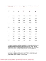
TABLE 6.1 State space density.










Mean density

Specific area density








Sample 1




20





40





Sample 2

10





20





Combined




30





60

This table shows the actual number of data points in two samples representative of the
same population. The specific area density in each sample is twice the mean density even
though the number of points in each sample is different. When the two samples are
combined, the combined state space still has the same relative specific area density as
each of the original state spaces. So it is that when looking at the density of a particular
volume of space, it is relative density that is most usefully examined.



Please purchase PDF Split-Merge on www.verypdf.com to remove this watermark.