- Trang chủ >>
- Khoa Học Tự Nhiên >>
- Vật lý
Ebook Spectrum Techniques Lab Manual Student Version
Bạn đang xem bản rút gọn của tài liệu. Xem và tải ngay bản đầy đủ của tài liệu tại đây (825.22 KB, 119 trang )
Spectrum Techniques
Lab Manual
Student Version
Revised, March 2011
Table of Contents
Student Usage of this Lab Manual ................................................. 3
What is Radiation? ......................................................................... 4
Introduction to Geiger-Müller Counters .......................................... 8
Good Graphing Techniques ......................................................... 10
Experiments
1.
2.
3.
4.
5.
6.
7.
8.
9.
10.
11.
12.
13.
Plotting a Geiger Plateau .............................................. 12
Statistics of Counting ................................................... 20
Background ................................................................... 26
Resolving Time ............................................................. 30
Geiger Tube Efficiency.................................................. 37
Shelf Ratios................................................................... 43
Backscattering............................................................... 48
Inverse Square Law ...................................................... 57
Range of Alpha Particles............................................... 62
Absorption of Beta Particles.......................................... 69
Beta Decay Energy ....................................................... 74
Absorption of Gamma Rays .......................................... 80
Half-Life of Ba-137m ..................................................... 88
Appendices
A.
B.
C.
D.
E.
F.
SI Units ......................................................................... 99
Common Radioactive Sources.................................... 101
Statistics...................................................................... 102
Radiation Passing Through Matter.............................. 109
Suggested References................................................ 113
NRC Regulations ........................................................ 116
Spectrum Techniques Student Lab Manual
2
Student Usage of Lab Manual
This manual is written to help students learn as much as possible about radiation
and some of the concepts key to nuclear and particle physics. This manual in particular
is written to guide you through a laboratory experiment set-up. The lab manual has the
following layout:
•
Detailed background material on radiation, the Geiger-Müller counter and its
operation, and radiation interaction with matter.
•
Thirteen laboratory experiments with instructions, data sheets, and analysis
instruction.
A piece of standalone equipment from Spectrum Techniques may not be entirely
equipped for the laboratory environment. Additional resources and recommendations
are made in the teacher’s notes of the experimental write-ups for schools that wish to
run the specific experiments. Also, schools operate on different class schedules,
varying from 42-minute periods to 3-hour lab sessions. Thus, the labs are written with
flexibility to combine them in different manners (our suggestions are listed below).
The lab manual is not intended to be a “recipe” book but a guide on how to obtain
the data and analyze it to answer certain questions. What this means is that explicit
directions as to every single button to push are not given, but the student will have
guidance where this can be inferred.
NOTE: All directions in this laboratory manual assume the use of a PC computer
with Microsoft Excel® used for the experiments. Any manual operation has the
appropriate directions given in the product manual. All operations listed in the directions
below may be carried out on the screen of the Spectrum Techniques equipment. Also,
all instructions use the ST-360 model Geiger-Müller counter, but the other models, ST160 and ST-260, have similar functions available.
Spectrum Techniques Student Lab Manual
3
What is Radiation?
This section will give you some of the basic information from a quick guide of the
history of radiation to some basic information to ease your mind about working with
radioactive sources. More information is contained in the introduction parts of the
laboratory experiments in this manual.
Historical Background
Radiation was discovered in the late 1800s. Wilhelm Röntgen observed
undeveloped photographic plates became exposed while he worked with high voltage
arcs in gas tubes, similar to a fluorescent light. Unable to identify the energy, he called
them “X” rays. The following year, 1896, Henri Becquerel observed that while working
with uranium salts and photographic plates, the uranium seemed to emit a penetrating
radiation similar to Röntgen’s X-rays. Madam Curie called this phenomenon
“radioactivity”. Further investigations by her and others showed that this property of
emitting radiation is specific to a given element or isotope of an element. It was also
found that atoms producing these radiations are unstable and emit radiation at
characteristic rates to form new atoms.
Atoms are the smallest unit of matter that retains the properties of an element
(such as hydrogen, carbon, or lead). The central core of the atom, called the nucleus, is
made up of protons (positive charge) and neutrons (no charge). The third part of the
atom is the electron (negative charge), which orbits the nucleus. In general, each atom
has an equal amount of protons and electrons so that the atom is electrically neutral.
The atom is made of mostly empty space. The atom’s size is on the order of an
angstrom (1 Å), which is equivalent to 1x10⁻¹⁰ m while the nucleus has a diameter of a
few fermis, or femtometers, which is equivalent to 1x10-15 m. This means that the
nucleus only occupies approximately 1/10,000 of the atom’s size. Yet, the nucleus
controls the atom’s behavior with respect to radiation. (The electrons control the
chemical behavior of the atom.)
Spectrum Techniques Student Lab Manual
4
Radioactivity
Radioactivity is a property of certain atoms to spontaneously emit particles or
electromagnetic wave energy. The nuclei of some atoms are unstable, and eventually
adjust to a more stable form by emission of radiation. These unstable atoms are called
radioactive atoms or isotopes. Radiation is energy emitted from radioactive atoms,
either as electromagnetic (EM) waves or as particles. When radioactive (or unstable)
atoms adjust, it is called radioactive decay or disintegration. A material containing a
large number of radioactive atoms is called either a radioactive material or a radioactive
source. Radioactivity, or the activity of a radioactive source, is measured in units
equivalent to the number of disintegrations per second (dps) or disintegrations per
minute (dpm). One unit of measure commonly used to denote the activity of a
radioactive source is the Curie (Ci) where one Curie equals thirty seven billion
disintegrations per second.
1 Ci = 3.7x10¹⁰ dps = 2.2x10¹² dpm
The SI unit for activity is called the Becquerel (Bq) and one Becquerel is equal to one
disintegration per second.
1 Bq = 1 dps = 60 dpm
Origins of Radiation
Radioactive materials that we find as naturally occurring were created by:
1. Formation of the universe, producing some very long lived radioactive elements,
such as uranium and thorium.
2. The decay of some of these long-lived materials into other radioactive materials like
radium and radon.
3. Fission products and their progeny (decay products), such as xenon, krypton, and
iodine.
Man-made radioactive materials are most commonly made as fission products or
from the decays of previously radioactive materials. Another method to manufacture
Spectrum Techniques Student Lab Manual
5
radioactive materials is activation of non-radioactive materials when they are
bombarded with neutrons, protons, other high-energy particles, or high-energy
electromagnetic waves.
Exposure to Radiation
Everyone on the face of the Earth receives background radiation from natural
and man-made sources. The major natural sources include radon gas, cosmic
radiation, terrestrial sources, and internal sources. The major man-made sources are
medical/dental sources, consumer products, and other (nuclear bomb and disaster
sources).
Radon gas is produced from the decay of uranium in the soil. The gas migrates
up through the soil, attaches to dust particles, and is breathed into our lungs. The
average yearly dose in the United States is about 200 mrem/yr. Cosmic rays are
received from outer space and our sun. The amount of radiation depends on where you
live; lower elevations receive less (~25 mrem/yr) while higher elevations receive more
(~50 mrem/yr). The average yearly dose in the United States is about 28 mrem/yr.
Terrestrial sources are sources that have been present from the formation of the Earth,
like radium, uranium, and thorium. These sources are in the ground, rock, and building
materials all around us. The average yearly dose from these sources in the United
States is about 28 mrem/yr. The last naturally occurring background radiation source is
due to the various chemicals in our own bodies. Potassium (40K) is the major
contributor and the average yearly dose in the United States is about 40 mrem/yr.
Background radiation can also be received from man-made sources. The most
common is the radiation from medical and dental x-rays. There is also radiation used to
treat cancer patients. The average yearly dose in the United States is about 54
mrem/yr. There are small amounts of radiation in consumer products, such as smoke
detectors, some luminous dial watches, and ceramic dishes (with an orange glaze). The
average yearly dose in the United States is about 10 mrem/yr. The other man-made
sources are fallout from nuclear bomb testing and usage, and from accidents such as
Chernobyl. That average yearly dose in the United States is about 3 mrem/yr.
Spectrum Techniques Student Lab Manual
6
Adding up the naturally occurring and man-made sources, we receive on
average about 360 mrem/yr of radioactivity exposure. What significance does this
number have since millirems have not been discussed yet? Without overloading you
with too much information, the government states the safety level for radiation exposure
5,000 mrem/yr. (This is the Department of Energy’s Annual Limit.) This is three times
below the level of exposure for biological damage to occur. So just living another year
(celebrating your birthday), you receive about 7% of the government regulated radiation
exposure. If you have any more questions, please ask your teacher.
Spectrum Techniques Student Lab Manual
7
The Geiger-Müller Counter
Geiger-Müller (GM) counters were invented by H. Geiger and E.W. Müller in
1928, and are used to detect radioactive particles (α and β) and rays (γ and x). A GM
tube usually consists of an airtight metal cylinder closed at both ends and filled with a
gas that is easily ionized (usually neon, argon, and halogen). One end consists of a
“window” which is a thin material, mica, allowing the entrance of alpha particles. (These
particles can be shielded easily.) A wire, which runs lengthwise down the center of the
tube, is positively charged with a relatively high voltage and acts as an anode. The tube
acts as the cathode. The anode and cathode are connected to an electric circuit that
maintains the high voltage between them.
When radiation enters the GM tube, it will ionize some of the atoms of the gas*.
Due to the large electric field created between the anode and cathode, the resulting
positive ions and negative electrons accelerate toward the cathode and anode,
respectively. Electrons move or drift through the gas at a speed of about 104 m/s, which
is about 104 times faster than the positive ions move. The electrons are collected a few
microseconds after they are created, while the positive ions would take a few
milliseconds to travel to the cathode. As the electrons travel toward the anode they
ionize other atoms, which produces a cascade of electrons called gas multiplication or a
(Townsend) avalanche. The multiplication factor is typically 106 to 108. The resulting
discharge current causes the voltage between the anode and cathode to drop. The
counter (electric circuit) detects this voltage drop and recognizes it as a signal of a
particle’s presence. There are additional discharges triggered by UV photons liberated
in the ionization process that start avalanches away from the original ionization site.
These discharges are called Geiger-Müller discharges. These do not effect the
performance as they are short-lived.
Now, once you start an avalanche of electrons how do you stop or quench it?
The positive ions may still have enough energy to start a new cascade. One (early)
method was external quenching, which was done electronically by quickly ramping
down the voltage in the GM tube after a particle was detected. This means any more
Spectrum Techniques Student Lab Manual
8
electrons or positive ions created will not be accelerated towards the anode or cathode,
respectively. The electrons and ions would recombine and no more signals would be
produced.
The modern method is called internal quenching. A small concentration of a
polyatomic gas (organic or halogen) is added to the gas in the GM tube. The quenching
gas is selected to have a lower ionization potential (~10 eV) than the fill gas (26.4 eV).
When the positive ions collide with the quenching gas’s molecules, they are slowed or
absorbed by giving its energy to the quenching molecule. They break down the gas
molecules in the process (dissociation) instead of ionizing the molecule. Any quenching
molecule that may be accelerated to the cathode dissociates upon impact producing no
signal. If organic molecules are used, GM tubes must be replaced as they permanently
break down over time (after about one billion counts). However, the GM tubes included
in Spectrum Techniques® set-ups use a halogen molecule, which naturally recombines
after breaking apart.
For any more specific details, we will refer the reader to literature such as G.F.
Knoll’s Radiation Detection and Measurement (John Wiley & Sons) or to Appendix E of
this lab manual.
A γ-ray interacts with the wall of the GM tube (by Compton scattering or photoelectric effect) to produce
an electron that passes to the interior of the tube. This electron ionizes the gas in the GM tube.
*
Spectrum Techniques Student Lab Manual
9
Physics Lab
Good Graphing Techniques
Very often, the data you take in the physics lab will require graphing. The following are a few
general instructions that you will find useful in creating good, readable, and usable graphs.
Further information on data analysis are given within the laboratory write-ups and in the
appendices.
1. Each graph MUST have a TITLE.
2. Make the graph fairly large – use a full sheet of graph paper for each graph. By
using this method, your accuracy will be better, but never more accurate that the
data originally taken.
3. Draw the coordinate axes using a STRAIGHT EDGE. Each coordinate is to be
labeled including units of the measurement.
4. The NUMERICAL VALUE on each coordinate MUST INCREASE in the direction
away from the origin.
Choose a value scale for each coordinate that is easy to work with. The range of the
values should be appropriate for the range of your data.
It is NOT necessary to write the numerical value at each division on the coordinate.
It is sufficient to number only a few of the divisions. DO NOT CLUTTER THE
GRAPH.
5. Circle each data point that you plot to indicate the uncertainty in the data
measurement.
Spectrum Techniques Student Lab Manual
10
6. CONNECT THE DATA POINTS WITH A BEST-FIT SMOOTH CURVE unless an
abrupt change in the slope is JUSTIFIABLY indicated by the data.
DO NOT PLAY CONNECT-THE-DOTS with your data! All data has some
uncertainty. Do NOT over-emphasize that uncertainty by connecting each point.
7. Determine the slope of your curve:
(a) Draw a slope triangle – use a dashed line.
(b) Your slope triangle should NOT intersect any data points, just the best-fit curve.
(c) Show your slope calculations right on the graph, e.g.,
slope =
∆ y y 2 − y1
= answer
=
∆x x 2 − x1
BE CERTAIN TO INCLUDE THE UNITS IN YOUR SLOPE CALCULATIONS.
8. You may use pencil to draw the graph if you wish.
9. Remember: NEATNESS COUNTS.
Spectrum Techniques Student Lab Manual
11
Lab #1: Plotting a GM Plateau
Objective:
In this experiment, you will determine the plateau and optimal operating voltage
of a Geiger-Müller counter.
Pre-lab Questions:
1. What will your graph look like (what does the plateau look like)?
2. Read the introduction section on GM tube operation. How does electric potential
effect a GM tube’s operation?
Introduction:
All Geiger-Müller (GM) counters do not operate in the exact same way because
of differences in their construction. Consequently, each GM counter has a different high
voltage that must be applied to obtain optimal performance from the instrument.
If a radioactive sample is positioned beneath a tube and the voltage of the GM
tube is ramped up (slowly increased by small intervals) from zero, the tube does not
start counting right away. The tube must reach the starting voltage where the electron
“avalanche” can begin to produce a signal. As the voltage is increased beyond that
point, the counting rate increases quickly before it stabilizes. Where the stabilization
begins is a region commonly referred to as the knee, or threshold value. Past the knee,
increases in the voltage only produce small increases in the count rate. This region is
the plateau we are seeking. Determining the optimal operating voltage starts with
identifying the plateau first. The end of the plateau is found when increasing the voltage
produces a second large rise in count rate. This last region is called the discharge
region.
To help preserve the life of the tube, the operating voltage should be selected
near the middle but towards the lower half of the plateau (closer to the knee). If the GM
tube operates too closely to the discharge region, and there is a change in the
Spectrum Techniques Student Lab Manual
12
performance of the tube. Then you could possibly operate the tube in a “continuous
discharge” mode, which can damage the tube.
Geiger Plataeu
14000
12000
Counts
10000
8000
6000
4000
2000
70
0
75
0
80
0
85
0
90
0
95
0
10
00
10
50
11
00
11
50
0
High Voltage (Volts)
Figure 1: A plateau graph for a Geiger-Müller counter.
By the end of this experiment, you will make a graph similar to the one in Figure 1,
which shows a typical plateau shape.
Equipment
•
Set-up for ST-360 Counter with GM Tube and stand (Counter box, power
supply – transformer, GM Tube, shelf stand, USB cable, and a source holder
for the stand) as shown in Figure 2.
•
Radioactive Source (e.g., Cs-137, Sr-90, or Co-60) – One of the orange, blue,
or green sources shown above in Figure 2.
Spectrum Techniques Student Lab Manual
13
Figure 2: ST360 setup with sources and absorber kit.
Procedure:
1. Plug in the transformer/power supply into any normal electricity outlet and into
the back of the ST-360 box. Next, remove the red or black end cap from the GM
tube VERY CAREFULLY. (Do NOT touch the thin window!) Place the GM
tube into the top of the shelf stand with the window down and BNC connector up.
Next, attach the BNC cable to the GM tube and the GM input on the ST-360.
Finally, attach the USB cable to the ST-360 and a USB port on your PC (if you
are using one).
2. Turn the power switch on the back of the ST-360 to the ON position, and double
click the STX software icon to start the program. You should then see the blue
control panel appear on your screen.
3. Go to the Setup menu and select the HV Setting option. In the High Voltage
(HV) window, start with 700 Volts. In the Step Voltage window, enter 20. Under
Spectrum Techniques Student Lab Manual
14
Enable Step Voltage, select On (the default selection is off). Finally, select
Okay.
4. Go under the Preset option and select Time. Enter 30 for the number of
seconds and choose OK. Then also under the Preset option choose Number of
Runs. In the window, enter 26 for the number of runs to make.
5. You should see a screen with a large window for the number of Counts and
Data for all the runs on the left half of the screen. On the right half, you should
see a window for the Preset Time, Elapsed Time, Runs Remaining, and High
Voltage. If not, go to the view option and select Scaler Counts. See Figure 1,
below.
Figure 1, STX setup for GM experiment
6. Make sure no other previous data by choosing the Erase All Data button (with
the red “X” or press F3). Then select the green diamond to start taking data.
7. When all the runs are taken, choose the File menu and Save As. Then you may
save the data file anywhere on the hard drive or onto a floppy disk. The output
file is a text file that is tab delimited, which means that it will load into most
Spectrum Techniques Student Lab Manual
15
spreadsheet programs. See the Data Analysis section for instructions in doing
the data analysis in Microsoft Excel®. Another option is that you may record the
data into your own data sheet and graph the data on the included graph paper.
8. You can repeat the data collection again with different values for step voltage
and duration of time for counting. However, the GM tubes you are using are not
allowed to have more than 1200 V applied to them. Consider this when choosing
new values.
Data Analysis
1. Open Microsoft Excel®. From the File Menu, choose Open. Find the directory
where you saved your data file. (The default location is on the C drive in the
SpecTech directory.) You will have to change the file types to All Files (*.*) to
find your data file that ends with .tsv. Then select your file to open it.
2. The Text Import Wizard will appear to step you through opening this file. You
may use any of the options available, but you need only to press Next, Next, and
Finish to open the file with all the data.
3. To see all the words and eliminate the ### symbols, you should expand the width
of the A and E columns. Place the cursor up to where the letters for the columns
are located. When the cursor is on the line between two columns, it turns into a
line with arrows pointing both ways. Directly over the lines between the A and B
columns and E and F columns, double-click and the columns should
automatically open to the maximum width needed.
4. To make a graph of this data, you may plot it with Excel® or on a sheet of graph
paper. If you choose Excel, the graphing steps are provided.
5. Go the Insert Menu and choose Chart for the Chart Wizard, or select it from the
top toolbar (it looks like a bar graph with different color bars).
6. Under Chart Types, select XY (Scatter) and choose Next. (This default
selection for a scatter plot is what we want to use.)
7. For the Data range, you want the settings to be on “=[your file
name]!$B$13:$C$32”, putting the name you chose for the data file in where [your
file name] is located (do not insert the square brackets or quotation marks). Also,
Spectrum Techniques Student Lab Manual
16
you want to change the Series In option from Rows to Columns. To check to
see if everything has worked, you should have a preview graph with only one set
of points on it. Or you can go to the Series Tab and for X Values should be
“=[your file name]!$B$13:$B$32” and for Y Values should be “=[your file
name]!$C$13:$C$32”. If this is correct, then choose Next again.
8. Next, you are given windows to insert a graph title and labels for the x and yaxes. Recall that we are plotting Counts on the y-axis and Voltage on the xaxis. When you have completed that, choose the Legend tab and unmark the
Show Legend Option (remove the check mark by clicking on the box). A legend
is not needed here unless you plotting more than one set of runs together.
9. Next, you are asked to choose whether to keep the graph as a separate
worksheet or to shrink it and insert it onto your current worksheet. This choice is
up to your instructor or you depending on how you want to choose your data
presentation for any lab report.
10. If you insert the chart onto the spreadsheet, adjust its size to print properly. Or
adjust the settings in the Print Preview Option (to the right of print on the top
toolbar).
Conclusions:
Now that you have plotted the GM tube’s plateau, what remains is to determine
an operating voltage. You should choose a value near the middle of the plateau or
slightly left of what you determine to be the center. Again, this will be somewhat difficult
due to the fact that you may not be able to see where the discharge region begins.
Post-Lab Questions:
1. The best operating voltage for the tube =
Volts.
2. Will this value be the same for all the different tubes in the lab?
3. Will this value be the same for this tube ten years from now?
4. One way to check to see if your operating voltage is on the plateau is to find the
slope of the plateau with your voltage included. If the slope for a GM plateau is less
Spectrum Techniques Student Lab Manual
17
than 10% per 100 volt, then you have a “good” plateau. Determine where your
plateau begins and ends, and confirm it is a good plateau. The equation for slope is
slope (% ) =
100(R2 − R1 ) / R1
× 100 ,
V2 − V1
where R1 and R2 are the activities for the beginning and end points, respectively. V1
and V2 and the voltages for the beginning and end points, respectively. (This equation
measures the % change of the activities and divides it by 100 V.)
Spectrum Techniques Student Lab Manual
18
Name:
Lab Session:
Date:
Partner:
Data Table for Geiger Plateau Lab
Tube #
Voltage
Counts
Voltage
Counts
Don’t forget to hand in this data sheet with a graph of the data.
Spectrum Techniques Student Lab Manual
19
Lab #2: Statistics of Counting
Objective:
In this experiment, the student will investigate the statistics related to
measurements with a Geiger counter. Specifically, the Poisson and Gaussian
distributions will be compared.
Pre-lab Questions:
1. List the formulas for finding the means and standard deviations for the
Poisson and Gaussian distribution.
2. A student in a previous class of the author’s once made the comment, “Why
do we have to learn about errors? You should just buy good and accurate
equipment.” How would you answer this student?
Introduction:
Statistics is an important feature especially when exploring nuclear and particle
physics. In those fields, we are dealing with very large numbers of atoms
simultaneously. We cannot possibly deal with each one individually, so we turn to
statistics for help. Its techniques help us obtain predictions on behavior based on what
most of the particles do and how many follow this pattern. These two categories fit a
general description of mean (or average) and standard deviation.
A measurement counts the number of successes resulting from a given number
of trials. Each trial is assumed to be a binary process in that there are two possible
outcomes: trial is a success or trial is not a success. For our work, the probability of a
decay or non-decay is a constant in every moment of time. Every atom in the source
has the same probability of decay, which is very small (you can measure it in the Halflife experiment).
The Poisson and Gaussian statistical distributions are the ones that will be used
in this experiment and in future ones. A detailed introduction to those distributions can
be found in Appendix C of this manual.
Spectrum Techniques Student Lab Manual
20
Equipment
Figure 1: Setup for ST360 with sources and absorber kit
•
Set-up for ST-360 Counter with GM Tube and stand (Counter box, power
supply – transformer, GM Tube, shelf stand, USB cable, and a source holder
for the stand) – Shown in Figure 1.
•
Radioactive Source (Cs-137 is recommended – the blue source in Figure 1)
Procedure:
1. Setup the equipment as you did in the Experiment #1, and open the computer
interface. You should then see the blue control panel appear on your screen.
2. Go to the Preset menu to preset the Time to 5 and Runs to 150.
3. Take a background radiation measurement. (This run lasts twelve and half minutes
to match the later measurements.)
4. When you are done, save your data onto disk (preferred for 150 data points).
Spectrum Techniques Student Lab Manual
21
5. Repeat with a Cesium-137 source, but reset the Time to 1 and the Number of Runs
to 750 (again will be twelve and a half minutes.)
Data Analysis
1. Open Microsoft Excel®. Import or enter all of your collected data.
2. First, enter all of the titles for numbers you will calculate. In cell G10, enter Mean.
In cell G13, enter Minimum. In cell G16, enter Maximum. In cell G19, enter
Standard Deviation. In cell G22, enter Square Root of Mean. In cell H10, enter
N. In cell I10, enter Frequency. In cell J10, enter Poisson Dist. Finally, in cell
K10, enter Gaussian Dist.
3. In cell G11, enter =AVERAGE(C12:C161) – this calculates the average, or mean.
4. In cell G14, enter =MIN(C12:C161) – this finds the smallest value of the data.
5. In cell G17, enter =MAX(C12:C161) – this finds the largest value of the data.
6. In cell G20, enter =STDEV(C12:C161) – this finds the standard deviation of the data.
7. In cell G22, enter =SQRT(G11) – this takes a square root of the value of the
designated cell, here G11.
8. Starting in cell H11, list the minimum number of counts recorded (same as
Minimum), which could be zero. Increase the count by one all the way down until
you reach the maximum number of counts.
9. In column I, highlight the empty cells that correspond to N values from column H.
Then from the Insert menu, choose function. A window will appear, you will want
to choose the FREQUENCY option that can be found under Statistical (functions
listed in alphabetical order). Once you choose Frequency, another window will
appear. In the window for Data Array, enter C12:C161 (cells for the data). In the
window for Bin Array, enter the cells for the N values in column H. (You can
highlight them by choosing the box at the end of the window.) STOP HERE!! If you
hit OK here, the function will not work. You must simultaneously choose, the
Control key, the Shift key, and OK button (on the screen). Then the frequency for
all of your N values will be computed. If you did not do it correctly, only the first
frequency value will be displayed.
Spectrum Techniques Student Lab Manual
22
10. In cell J11, enter the formula =$G$11^H11/FACT(H11)*EXP(-$G$11)*150 for the
Poisson Distribution. (You must multiply the standard formula by 150, because
the standard formula is normalized to 11.)
11. In cell K11, enter the formula =(1/($G$20*SQRT(2*PI())))*EXP(-((H11$G$11)^2)/(2*$G$20^2))*150 for the Gaussian Distribution. Note that in Excel®
the number π is represented by PI(). Again, you must multiply by 150 to let the
function know how many entries there are. (NOTE: The formula this is derived from
can be found in Appendix C.)
12. Next, make a graph of all three distributions: Raw Frequency, Poisson
Distribution, and Gaussian Distribution. Start with the Chart Wizard either by
choosing Chart 8 from the Insert Menu or pressing its icon on the top toolbar. (See
Lab #1 if you need more detailed instructions.)
13. For your graph, select the N values in the H column and the Frequency values in the
I column. Now add two more series, one for the Poisson Distribution and one for
the Gaussian Distribution.
14. Print the graph to hand in to your instructor.
15. Repeat this whole data analysis procedure for your counts with Cs-137.
Conclusions:
What you have plotted is the frequency plot for your data. In addition, you have
plotted on top of them the predictions of a Poisson and Gaussian Distribution. (Note:
for the Cs-137 data, the Poisson distribution will read #NUM, because the number is too
high for Excel® to deal with, even in scientific notation.) How well do the statistical
distributions predict the data? How close are the standard deviations? Is one better
than the other? Do the conditions of when to use the Gaussian or Poisson
Distributions apply correctly for our data?
1
Normalization is a common higher math procedure. One common technique is to make the highest value 1
and scale all the data below it.
Spectrum Techniques Student Lab Manual
23
Post-Lab Questions:
1. Which distribution matches the data with the background counts? How well does
the Gaussian distribution describe the Cs-137 data?
2. Why can’t you get a value for the Poisson distribution with the data from the
Cesium-137 source?
3. How close are the standard deviation values when calculated with the Poisson and
Gaussian Distributions? Is one right (or more correct)? Is one easier to calculate?
Spectrum Techniques Student Lab Manual
24
Name:
Lab Session:
Date:
Partner:
Data Sheet for Statistics Lab
Tube #:
Source:
Run Duration:
Tube #:
Source:
Run Duration:
(Time)
(Time)
Run #
Counts
Data Set
Mean
Run #
Gaussian σ
Counts
Poisson σ
Background
Cs-137
Don’t forget to hand in this data sheet with a graph of the data.
Spectrum Techniques Student Lab Manual
25