Ebook Basic engineering mathematics (4th edition) Part 2
Bạn đang xem bản rút gọn của tài liệu. Xem và tải ngay bản đầy đủ của tài liệu tại đây (5.48 MB, 172 trang )
16
Reduction of non-linear laws to linear form
16.1 Determination of law
Frequently, the relationship between two variables, say x and y,
is not a linear one, i.e. when x is plotted against y a curve results.
In such cases the non-linear equation may be modified to the
linear form, y = mx + c, so that the constants, and thus the law
relating the variables can be determined. This technique is called
‘determination of law’.
Some examples of the reduction of equations to linear form
include:
(i) y = ax2 + b compares with Y = mX + c, where m = a, c = b
and X = x2 .
Hence y is plotted vertically against x2 horizontally to
produce a straight line graph of gradient ‘a’ and y-axis
intercept ‘b’
a
(ii) y = + b
x
1
y is plotted vertically against horizontally to produce a
x
straight line graph of gradient ‘a’ and y-axis intercept ‘b’
(iii) y = ax2 + bx
y
= ax + b.
x
y
Comparing with Y = mX + c shows that is plotted vertix
cally against x horizontally to produce a straight line graph
y
of gradient ‘a’ and axis intercept ‘b’
x
If y is plotted against x a curve results and it is not possible
to determine the values of constants a and b from the curve.
Comparing y = ax2 + b with Y = mX + c shows that y is to be
plotted vertically against x2 horizontally. A table of values is
drawn up as shown below.
x
x2
y
1
1
9.8
2
4
15.2
3
9
24.2
4
16
36.5
5
25
53.0
A graph of y against x2 is shown in Fig. 16.1, with the best straight
line drawn through the points. Since a straight line graph results,
the law is verified.
y
53
50
A
40
30
Dividing both sides by x gives
Problem 1. Experimental values of x and y, shown
below, are believed to be related by the law
y = ax2 + b. By plotting a suitable graph verify this
law and determine approximate values of a and b.
20
17
B
C
10
8
0
5
10
15
20
25
Fig. 16.1
x
y
1
9.8
2
15.2
3
24.2
4
36.5
5
53.0
From the graph, gradient a =
AB 53 − 17 36
=
=
= 1.8
BC
25 − 5
20
x2
118
Basic Engineering Mathematics
and the y-axis intercept, b = 8.0
Hence the law of the graph is y = 1.8x 2 + 8.0
35
Problem 2. Values of load L newtons and distance d metres
obtained experimentally are shown in the following table.
31
30
A
25
Load, L N
distance, d m
32.3
0.75
29.6
0.37
Load, L N
distance, d m
18.3
0.12
12.8
0.09
27.0
0.24
10.0
0.08
23.2
0.17
L 20
6.4
0.07
15
Verify that load and distance are related by a law of the
a
form L = + b and determine approximate values of a and
d
b. Hence calculate the load when the distance is 0.20 m and
the distance when the load is 20 N.
11
10
1
horizontally.
d
Another table of values is drawn up as shown below.
32.3 29.6 27.0 23.2 18.3 12.8 10.0
0.75 0.37 0.24 0.17 0.12 0.09 0.08
1.33
2.70
4.17
5.88
6.4
0.07
8.33 11.11 12.50 14.29
1
is shown in Fig. 16.2. A straight line can
d
be drawn through the points, which verifies that load and distance
a
are related by a law of the form L = + b.
d
AB 31 − 11
=
Gradient of straight line, a =
BC
2 − 12
20
= −2
=
−10
L-axis intercept,
b = 35
A graph of L against
2
Hence the law of the graph is L = − + 35
d
When the distance d = 0.20 m,
load L =
−2
+ 35 = 25.0 N
0.20
Rearranging L = −
2
+ 35 gives
d
2
= 35 − L
d
and
d=
2
35 − L
Hence when the load L = 20 N,
distance d =
2
4
6
+ b with Y = mX + c
shows that L is to be plotted vertically against
L
d
1
d
C
5
0
1
a
Comparing L = + b i.e. L = a
d
d
B
2
2
=
= 0.13 m
35 − 20
15
8
1
d
10
12
14
Fig. 16.2
Problem 3. The solubility s of potassium chlorate is shown
by the following table:
t◦C
s
10 20 30 40 50 60 80 100
4.9 7.6 11.1 15.4 20.4 26.4 40.6 58.0
The relationship between s and t is thought to be of the form
s = 3 + at + bt 2 . Plot a graph to test the supposition and
use the graph to find approximate values of a and b. Hence
calculate the solubility of potassium chlorate at 70◦ C.
Rearranging s = 3 + at + bt 2 gives s − 3 = at + bt 2 and
s−3
= a + bt
t
or
s−3
= bt + a
t
s−3
is to be
t
plotted vertically and t horizontally. Another table of values is
drawn up as shown below.
which is of the form Y = mX + c, showing that
t
10 20 30
40
50
60
80
100
s
4.9 7.6 11.1 15.4 20.4 26.4 40.6 58.0
s−3
0.19 0.23 0.27 0.31 0.35 0.39 0.47 0.55
t
s−3
against t is shown plotted in Fig. 16.3.
t
A straight line fits the points which shows that s and t are
related by s = 3 + at + bt 2 .
Gradient of straight line,
A graph of
b=
0.39 − 0.19
0.20
AB
=
=
= 0.004
BC
60 − 10
50
Reduction of non-linear laws to linear form
and find the approximate values for a and b. Determine
the cross-sectional area needed for a resistance reading
of 0.50 ohms.
0.6
0.5
sϪ3
t
7. Corresponding experimental values of two quantities x
and y are given below.
0.4
0.39
A
x
y
0.3
0.2
0.19
0.15
0.1
119
0
20
40
60
80
t °C
100
Fig. 16.3
Vertical axis intercept, a = 0.15
Hence the law of the graph is s = 3 + 0.15t + 0.004t 2
The solubility of potassium chlorate at 70◦ C is given by
2
= 3 + 10.5 + 19.6 = 33.1
0.89
1.75
9.0
169.0
0.76
2.04
2.0
2.8
3.6
4.2
4.8
475
339
264
226
198
9. The following results give corresponding values of two
quantities x and y which are believed to be related by a
law of the form y = ax2 + bx where a and b are constants.
33.86
3.4
55.54
5.2
72.80
6.5
84.10
7.3
111.4
9.1
168.1
12.4
Hence determine (i) the value of y when x is 8.0 and
(ii) the value of x when y is 146.5.
In Problems 1 to 5, x and y are two related variables and
all other letters denote constants. For the stated laws to be
verified it is necessary to plot graphs of the variables in a
modified form. State for each (a) what should be plotted on
the vertical axis, (b) what should be plotted on the horizontal
axis, (c) the gradient and (d) the vertical axis intercept.
√
2. y − a = b x
1. y = d + cx2
f
4. y − cx = bx2
3. y − e =
x
a
5. y = + bx
x
6. In an experiment the resistance of wire is measured for
wires of different diameters with the following results.
1.14
1.42
7.5
119.5
Verify the law and determine approximate values of a
and b.
Exercise 60 Further problems on reducing
non-linear laws to linear form
(Answers on page 277)
1.64
1.10
6.0
79.0
It is believed that the relationship between load and span
is L = c/d, where c is a constant. Determine (a) the value
of constant c and (b) the safe load for a span of 3.0 m.
y
x
Now try the following exercise
R ohms
d mm
4.5
47.5
8. Experimental results of the safe load L kN, applied to
girders of varying spans, d m, are shown below.
Span, d m
Load, L kN
s = 3 + 0.15(70) + 0.004(70)
3.0
25.0
By plotting a suitable graph verify that y and x are connected by a law of the form y = kx2 + c, where k and c
are constants. Determine the law of the graph and hence
find the value of x when y is 60.0
B
C
1.5
11.5
0.63
2.56
It is thought that R is related to d by the law
R = (a/d 2 ) + b, where a and b are constants. Verify this
16.2 Determination of law involving
logarithms
Examples of reduction of equations to linear form involving
logarithms include:
(i) y = axn
Taking logarithms to a base of 10 of both sides gives:
lg y = lg (axn ) = lg a + lg xn
i.e. lg y = n lg x + lg a by the laws of logarithms
which compares with Y = mX + c
and shows that lg y is plotted vertically against lg x horizontally to produce a straight line graph of gradient n and
lg y-axis intercept lg a
120
Basic Engineering Mathematics
(ii) y = abx
Taking logarithms to a base of 10 of the both sides gives:
3.0
2.98
lg y = lg(abx )
i.e. lg y = lg a + lg bx
2.78
i.e. lg y = x lg b + lg a
or
A
D
by the laws of logarithms
lg P
lg y = ( lg b)x + lg a
2.5
which compares with Y = mX + c
and shows that lg y is plotted vertically against x horizontally
to produce a straight line graph of gradient lg b and lg y-axis
intercept lg a
2.18
(iii) y = aebx
2.0
0.30 0.40
Taking logarithms to a base of e of both sides gives:
ln y = ln(aebx )
i.e. ln y = ln a + bx ln e
i.e. ln y = bx + ln a
ln e = 1
n=
and shows that ln y is plotted vertically against x horizontally
to produce a straight line graph of gradient b and ln y-axis
intercept ln a
Problem 4. The current flowing in, and the power dissipated by, a resistor are measured experimentally for various
values and the results are as shown below.
3.6
311
4.1
403
5.6
753
6.8
1110
Show that the law relating current and power is of the
form P = RI n , where R and n are constants, and determine
the law.
Taking logarithms to a base of 10 of both sides of P = RI n gives:
lg P = lg(RI n ) = lg R + lg I n = lg R + n lg I
by the laws of logarithms,
i.e. lg P = n lg I + lg R, which is of the form Y = mX + c, showing that lg P is to be plotted vertically against lg I horizontally.
A table of values for lg I and lg P is drawn up as shown below.
2.2
0.342
116
2.064
3.6
0.556
311
2.493
0.70
0.80
0.90
Gradient of straight line,
since
2.2
116
0.60
lg l
which compares with Y = mX + c
Current, I amperes
Power, P watts
0.50
Fig. 16.4
i.e. ln y = ln a + ln ebx
I
lg I
P
lg P
B
C
4.1
0.613
403
2.605
5.6
0.748
753
2.877
6.8
0.833
1110
3.045
A graph of lg P against lg I is shown in Fig. 16.4 and since a
straight line results the law P = RI n is verified.
2.98 − 2.18
0.80
AB
=
=
=2
BC
0.8 − 0.4
0.4
It is not possible to determine the vertical axis intercept on sight
since the horizontal axis scale does not start at zero. Selecting any point from the graph, say point D, where lg I = 0.70
and lg P = 2.78, and substituting values into lg P = n lg I + lg R
gives
2.78 = (2)(0.70) + lg R
from which lg R = 2.78 − 1.40 = 1.38
Hence
R = antilog 1.38 (= 101.38 ) = 24.0
Hence the law of the graph is P = 24.0 I 2
Problem 5. The periodic time, T , of oscillation of a pendulum is believed to be related to its length, l, by a law of
the form T = kl n , where k and n are constants. Values of T
were measured for various lengths of the pendulum and the
results are as shown below.
Periodic time, T s
Length, l m
1.0 1.3 1.5 1.8 2.0 2.3
0.25 0.42 0.56 0.81 1.0 1.32
Show that the law is true and determine the approximate
values of k and n. Hence find the periodic time when the
length of the pendulum is 0.75 m.
From para (i), if T = kl n then
lg T = n lg l + lg k
and comparing with
Y = mX + c
Reduction of non-linear laws to linear form
shows that lg T is plotted vertically against lg l horizontally.
A table of values for lg T and lg l is drawn up as shown below.
T
lg T
l
lg l
1.0
1.3
1.5
1.8
0
0.114
0.176
0.255
0.25
0.42
0.56
0.81
−0.602 −0.377 −0.252 −0.092
2.0
0.301
1.0
0
2.3
0.362
1.32
0.121
A graph of lg T against lg l is shown in Fig. 16.5 and the law
T = kl n is true since a straight line results.
lg T
lg y = (lgb)x + lg a
and comparing with
Y = mX + c
shows that lg y is plotted vertically and x horizontally.
Another table is drawn up as shown below.
0
5.0
0.70
0.6
9.67
0.99
1.2
18.7
1.27
1.8
36.1
1.56
2.4
69.8
1.84
3.0
135.0
2.13
A graph of lg y against x is shown in Fig. 16.6 and since a
straight line results, the law y = abx is verified.
0.30
A
From para (ii), if y = abx then
x
y
lg y
0.40
121
0.25
2.50
0.20
2.13
2.00
A
C
lg y
0.10
0.05
B
1.50
Ϫ0.60 Ϫ0.50 Ϫ0.40 Ϫ0.30 Ϫ0.20 Ϫ0.10
0
0.10
0.20
lg I
1.17
B
C
Fig. 16.5
1.00
From the graph, gradient of straight line,
n=
0.25 − 0.05
0.20
1
AB
=
=
=
BC
−0.10 − (−0.50)
0.40
2
0.70
0.50
0
1.0
2.0
3.0
x
Vertical axis intercept, lg k = 0.30
Hence k = antilog 0.30 (= 100.30 ) = 2.0
√
Hence the law of the graph is T = 2.0 l 1/2 or T = 2.0 l
√
When length l = 0.75 m then T = 2.0 0.75 = 1.73 s
Problem 6. Quantities x and y are believed to be related
by a law of the form y = abx , where a and b are constants.
Values of x and corresponding values of y are:
x
y
0
5.0
0.6
9.67
1.2
18.7
1.8
36.1
2.4
69.8
3.0
135.0
Verify the law and determine the approximate values of
a and b. Hence determine (a) the value of y when x is 2.1
and (b) the value of x when y is 100
Fig. 16.6
Gradient of straight line,
lg b =
2.13 − 1.17
0.96
AB
=
=
= 0.48
BC
3.0 − 1.0
2.0
Hence b = antilog 0.48 (= 100.48 ) = 3.0, correct to 2 significant
figures.
Vertical axis intercept, lg a = 0.70,
from which a = antilog 0.70 (= 100.70 )
= 5.0, correct to 2 significant figures
Hence the law of the graph is y = 5.0(3.0)x
122
Basic Engineering Mathematics
(a) When x = 2.1, y = 5.0(3.0)2.1 = 50.2
(b) When y = 100, 100 = 5.0(3.0)x ,
A
5.0
from which 100/5.0 = (3.0)x ,
20 = (3.0)x
i.e.
4.0
Taking logarithms of both sides gives
lg 20 = lg(3.0) = x lg 3.0
ln i
Hence x =
1.3010
lg 20
=
= 2.73
lg 3.0 0.4771
2.0
Problem 7. The current i mA flowing in a capacitor which
is being discharged varies with time t ms as shown below.
i mA
t ms
203
100
61.14
160
22.49
210
6.13
275
2.49
320
0.615
390
Show that these results are related by a law of the form
i = I et/T , where I and T are constants. Determine the
approximate values of I and T .
Taking Napierian logarithms of both sides of i = I et/T gives
ln i = ln (I et/T ) = ln I + ln et/T
160
61.14
4.11
210
22.49
3.11
275
6.13
1.81
320
2.49
0.91
390
0.615
−0.49
A graph of ln i against t is shown in Fig. 16.7 and since a straight
line results the law i = I et/T is verified.
Gradient of straight line,
1
AB
5.30 − 1.30
4.0
=
=
=
= −0.02
T
BC
100 − 300
−200
1
= −50
Hence T =
−0.02
Selecting any point on the graph, say point D, where t = 200 and
1
t + ln I gives
ln i = 3.31, and substituting into ln i =
T
1
(200) + ln I
50
ln I = 3.31 + 4.0 = 7.31
3.31 = −
from which
C
B
0
100
200
300
400 t (ms)
Ϫ1.0
Fig. 16.7
and I = antilog 7.31 (= e7.31 ) = 1495 or 1500 correct to 3 significant figures.
Now try the following exercise
which compares with y = mx + c, showing that ln i is plotted
vertically against t horizontally. (For methods of evaluating
Napierian logarithms see Chapter 15.) Another table of values
is drawn up as shown below.
100
203
5.31
1.30
1.0
Hence the law of the graph is i = 1500e−t/50
t
(since ln e = 1)
i.e. ln i = ln I +
T
1
t + ln I
or ln i =
T
t
i
ln i
D (200, 3.31)
3.31
3.0
x
Exercise 61
Further problems on reducing non-linear
laws to linear form (Answers on page 277)
In Problems 1 to 3, x and y are two related variables and
all other letters denote constants. For the stated laws to be
verified it is necessary to plot graphs of the variables in
a modified form. State for each (a) what should be plotted on the vertical axis, (b) what should be plotted on the
horizontal axis, (c) the gradient and (d) the vertical axis
intercept.
1. y = bax
2. y = kxl
3.
y
= enx
m
4. The luminosity I of a lamp varies with the applied voltage
V and the relationship between I and V is thought to be
I = kV n . Experimental results obtained are:
I candelas
V volts
1.92 4.32 9.72 15.87 23.52 30.72
40 60 90 115 140 160
Verify that the law is true and determine the law of
the graph. Determine also the luminosity when 75 V is
applied across the lamp.
Reduction of non-linear laws to linear form
5. The head of pressure h and the flow velocity v are
measured and are believed to be connected by the law
v = ahb , where a and b are constants. The results are as
shown below.
h
v
10.6
9.77
13.4
11.0
17.2
12.44
24.6
14.88
29.3
16.24
Verify that the law is true and determine values of a and b
6. Experimental values of x and y are measured as follows.
x
y
0.4
8.35
0.9
13.47
1.2
17.94
2.3
51.32
3.8
215.20
The law relating x and y is believed to be of the
form y = abx , where a and b are constants. Determine
the approximate values of a and b. Hence find the
value of y when x is 2.0 and the value of x when
y is 100
7. The activity of a mixture of radioactive isotope is
believed to vary according to the law R = R0 t −c , where
R0 and c are constants.
123
Experimental results are shown below.
R
t
9.72
2
2.65
5
1.15
9
0.47
17
0.32
22
0.23
28
Verify that the law is true and determine approximate
values of R0 and c.
8. Determine the law of the form y = aekx which relates the
following values.
y
x
0.0306
−4.0
0.285
5.3
0.841 5.21
9.8 17.4
173.2
32.0
1181
40.0
9. The tension T in a belt passing round a pulley wheel
and in contact with the pulley over an angle of θ radians
is given by T = T0 eµθ , where T0 and µ are constants.
Experimental results obtained are:
T newtons
θ radians
47.9 52.8 60.3 70.1
1.12 1.48 1.97 2.53
80.9
3.06
Determine approximate values of T0 and µ. Hence find
the tension when θ is 2.25 radians and the value of θ
when the tension is 50.0 newtons.
17
Graphs with logarithmic scales
17.1 Logarithmic scales
Graph paper is available where the scale markings along the horizontal and vertical axes are proportional to the logarithms of the
numbers. Such graph paper is called log–log graph paper.
1
2
3
4
5
6
7 8 9 10
Fig. 17.1
100
A
10
y ϭ ax b
y
A logarithmic scale is shown in Fig. 17.1 where the distance between, say 1 and 2, is proportional to lg 2 − lg 1, i.e.
0.3010 of the total distance from 1 to 10. Similarly, the distance
between 7 and 8 is proportional to lg 8 − lg 7, i.e. 0.05799 of the
total distance from 1 to 10. Thus the distance between markings
progressively decreases as the numbers increase from 1 to 10.
With log–log graph paper the scale markings are from 1 to
9, and this pattern can be repeated several times. The number
of times the pattern of markings is repeated on an axis signifies
the number of cycles. When the vertical axis has, say, 3 sets of
values from 1 to 9, and the horizontal axis has, say, 2 sets of
values from 1 to 9, then this log–log graph paper is called ‘log 3
cycle × 2 cycle’ (see Fig. 17.2). Many different arrangements are
available ranging from ‘log 1 cycle × 1 cycle’ through to ‘log 5
cycle × 5 cycle’.
To depict a set of values, say, from 0.4 to 161, on an axis of
log–log graph paper, 4 cycles are required, from 0.1 to 1, 1 to 10,
10 to 100 and 100 to 1000.
17.2 Graphs of the form y = ax n
Taking logarithms to a base of 10 of both sides of y = axn
gives:
1.0
lg y = lg(axn )
B
C
= lg a + lg xn
i.e.
which compares with
0.1
Fig. 17.2
1.0
x
10
lg y = n lg x + lg a
Y = mX + c
Thus, by plotting lg y vertically against lg x horizontally, a straight
line results, i.e. the equation y = axn is reduced to linear form.
With log–log graph paper available x and y may be plotted
directly, without having first to determine their logarithms,
as shown in Chapter 16.
Graphs with logarithmic scales
Problem 1. Experimental values of two related quantities
x and y are shown below:
x
y
0.41
0.45
0.63
1.21
0.92
2.89
1.36
7.10
2.17
20.79
Taking logarithms of both sides gives
lg 24.643 = b lg 4, i.e.
lg 24.643
lg 4
= 2.3, correct to 2 significant figures.
b=
3.95
82.46
The law relating x and y is believed to be y = axb , where a
and b are constants. Verify that this law is true and determine
the approximate values of a and b.
If y = ax then lg y = b lg x + lg a, from above, which is of the
form Y = mX + c, showing that to produce a straight line graph
lg y is plotted vertically against lg x horizontally. x and y may be
plotted directly on to log–log graph paper as shown in Fig. 17.2.
The values of y range from 0.45 to 82.46 and 3 cycles are
needed (i.e. 0.1 to 1, 1 to 10 and 10 to 100). The values of x
range from 0.41 to 3.95 and 2 cycles are needed (i.e. 0.1 to 1
and 1 to 10). Hence ‘log 3 cycle × 2 cycle’ is used as shown
in Fig. 17.2 where the axes are marked and the points plotted. Since the points lie on a straight line the law y = axb is
verified.
b
To evaluate constants a and b:
Method 1. Any two points on the straight line, say points A
and C, are selected, and AB and BC are measured (say in
centimetres).
Then, gradient, b =
125
AB 11.5 units
=
= 2.3
BC
5 units
Substituting b = 2.3 in equation (1) gives:
17.25 = a(2)2.3 , i.e.
17.25
17.25
=
(2)2.3
4.925
= 3.5, correct to 2 significant figures.
a=
Hence the law of the graph is: y = 3.5x2.3
Problem 2. The power dissipated by a resistor was
measured for varying values of current flowing in the
resistor and the results are as shown:
Current, I amperes
Power, P watts
1.4 4.7 6.8 9.1 11.2 13.1
49 552 1156 2070 3136 4290
Prove that the law relating current and power is of the form
P = RI n , where R and n are constants, and determine the law.
Hence calculate the power when the current is 12 amperes
and the current when the power is 1000 watts.
Since lg y = b lg x + lg a, when x = 1, lg x = 0 and lg y = lg a.
The straight line crosses the ordinate x = 1.0 at y = 3.5.
Hence lg a = lg 3.5, i.e. a = 3.5
Method 2. Any two points on the straight line, say points A
and C, are selected. A has coordinates (2, 17.25) and C has
coordinates (0.5, 0.7).
Since
y = axb then 17.25 = a(2)b
0.7 = a(0.5)b
and
(1)
(2)
i.e. two simultaneous equations are produced and may be solved
for a and b.
Since P = RI n then lg P = nlg l + lg R, which is of the form
Y = mX + c, showing that to produce a straight line graph lg P is
plotted vertically against lg I horizontally. Power values range
from 49 to 4290, hence 3 cycles of log–log graph paper are
needed (10 to 100, 100 to 1000 and 1000 to 10 000). Current
values range from 1.4 to 11.2, hence 2 cycles of log–log
graph paper are needed (1 to 10 and 10 to 100). Thus
‘log 3 cycles × 2 cycles’ is used as shown in Fig. 17.3 (or, if
not available, graph paper having a larger number of cycles
per axis can be used). The co-ordinates are plotted and a
straight line results which proves that the law relating current and power is of the form P = RI n . Gradient of straight
line,
n=
Dividing equation (1) by equation (2) to eliminate a gives:
17.25
(2)b
=
=
0.7
(0.5)b
i.e.
24.643 = (4)b
2
0.5
b
AB
14 units
=
=2
BC
7 units
At point C, I = 2 and P = 100. Substituting these values into
P = RI n gives: 100 = R(2)2 . Hence R = 100/(2)2 = 25 which
may have been found from the intercept on the I = 1.0 axis in
Fig. 17.3.
126
Basic Engineering Mathematics
Since p = cv n , then lg p = n lg v + lg c, which is of the form
Y = mX + c, showing that to produce a straight line graph lg
p is plotted vertically against lg v horizontally. The co-ordinates
are plotted on ‘log 3 cycle × 2 cycle’ graph paper as shown in
Fig. 17.4. With the data expressed in standard form, the axes are
marked in standard form also. Since a straight line results the law
p = cv n is verified.
10000
A
1000
Power, P watts
1 ϫ 108
Pϭ Rl n
A
B
C
10
1.0
1 ϫ 107
10
Current, l amperes
100
Pressure, p Pascals
100
p ϭ cv n
1 ϫ 106
Fig. 17.3
C
B
Hence the law of the graph is P = 25I 2
When current I = 12, power P = 25(12)2 = 3600 watts (which
may be read from the graph).
When power P = 1000, 1000 = 25I 2 .
Hence
from which,
1000
= 40,
25
√
I = 40 = 6.32 A
I2 =
p pascals
v m3
2.28 × 10⁵
3.2 × 10⁻²
1 ϫ 10Ϫ1
The straight line has a negative gradient and the value of the
gradient is given by:
8.04 × 10⁵
1.3 × 10⁻²
5.05 × 10⁶
3.5 × 10⁻³
1 ϫ 10Ϫ2
Volume, v m3
Fig. 17.4
Problem 3. The pressure p and volume v of a gas are
believed to be related by a law of the form p = cv n ,
where c and n are constants. Experimental values of p and
corresponding values of v obtained in a laboratory are:
p pascals
v m3
1 ϫ 105
1 ϫ 10Ϫ3
2.03 × 10⁶
6.7 × 10⁻³
1.82 × 10⁷
1.4 × 10⁻³
Verify that the law is true and determine approximate values
of c and n.
14 units
AB
=
= 1.4,
BC
10 units
hence n = −1.4
Selecting any point on the straight line, say point C, having
co-ordinates (2.63 × 10⁻² , 3 × 10⁵ ), and substituting these
values in p = cv n gives:
3×105 = c(2.63×10⁻² )−1.4
Hence
c=
3×10⁵
3×105
=
(2.63×10⁻² )−1.4 (0.0263)−1.4
3×10⁵
1.63×102
= 1840, correct to 3 significant figures.
=
Graphs with logarithmic scales
called log–linear graph paper, and is specified by the number of
cycles on the logarithmic scale. For example, graph paper having
3 cycles on the logarithmic scale is called ‘log 3 cycle × linear’
graph paper.
Hence the law of the graph is:
p = 1840υ −1.4
pυ 1.4 = 1840
or
Now try the following exercise
Exercise 62 Further problems on graphs of the form
y = ax n (Answers on page 277)
1. Quantities x and y are believed to be related by a
law of the form y = axn , where a and n are constants.
Experimental values of x and corresponding values
of y are:
x
y
0.8
8
2.3
54
5.4
250
11.5
974
21.6
3028
42.9
10 410
Show that the law is true and determine the values of a
and n. Hence determine the value of y when x is 7.5 and
the value of x when y is 5000.
2. Show from the following results of voltage V and admittance Y of an electrical circuit that the law connecting
the quantities is of the form V = kY n , and determine the
values of k and n.
Voltage,
V volts
Admittance
Y siemens
127
2.88
2.05
1.60
1.22
0.96
0.52
0.73
0.94
1.23
1.57
Problem 4. Experimental values of quantities x and y are
believed to be related by a law of the form y = abx , where
a and b are constants. The values of x and corresponding
values of y are:
x
y
0.7
18.4
1.4
45.1
2.1
111
2.9
308
3.7
858
4.3
1850
Verify the law and determine the approximate values of a
and b. Hence evaluate (i) the value of y when x is 2.5, and
(ii) the value of x when y is 1200.
Since y = abx then lg y = (lg b) x + lg a (from above), which is
of the form Y = mX + c, showing that to produce a straight line
graph lg y is plotted vertically against x horizontally. Using log–
linear graph paper, values of x are marked on the horizontal scale
to cover the range 0.7 to 4.3. Values of y range from 18.4 to 1850
and 3 cycles are needed (i.e. 10 to 100, 100 to 1000 and 1000 to
10 000). Thus ‘log 3 cycles × linear’graph paper is used as shown
in Fig. 17.5. A straight line is drawn through the co-ordinates,
hence the law y = abx is verified.
10000
3. Quantities x and y are believed to be related by a law
of the form y = mnx . The values of x and corresponding
values of y are:
x
y
0
1.0
0.5
3.2
1.0
10
1.5
31.6
2.0
100
2.5
316
3.0
1000
A
1000
y ϭ ab x
Verify the law and find the values of m and n.
17.3
Graphs of the form y = abx
Taking logarithms to a base of 10 of both sides of y = abx gives:
100
B
C
lg y = lg(abx ) = lg a + lg bx = lg a + xlg b
i.e.
which compares with
lg y = (lg b)x + lg a
Y = mX + c
Thus, by plotting lg y vertically against x horizontally a straight
line results, i.e. the graph y = abx is reduced to linear form. In
this case, graph paper having a linear horizontal scale and a logarithmic vertical scale may be used. This type of graph paper is
10
0
0.5
1.0
1.5
2.0
2.5
x
Fig. 17.5
3.0
3.5
4.0
4.5
128
Basic Engineering Mathematics
Gradient of straight line, lg b = AB/BC. Direct measurement
(say in centimetres) is not made with log-linear graph paper since
the vertical scale is logarithmic and the horizontal scale is linear.
Hence
lg 1000 − lg 100
3−2
AB
=
=
BC
3.82 − 2.02
1.80
1
=
= 0.5556
1.80
17.4 Graphs of the form y = aekx
Taking logarithms to a base of e of both sides of y = aekx
gives:
ln y = ln(aekx ) = ln a + ln ekx = ln a + kx ln e
ln y = kx + ln a (since ln e = 1)
i.e.
which compares with Y = mX + c
Hence b = antilog 0.5556(=100.5556 ) = 3.6, correct to 2 significant figures.
Point A has coordinates (3.82, 1000).
Substituting these values into y = abx gives:
1000 = a(3.6)3.82 , i.e.
Thus, by plotting ln y vertically against x horizontally, a straight
line results, i.e. the equation y = aekx is reduced to linear form.
In this case,. graph paper having a linear horizontal scale and a
logarithmic vertical scale may be used.
Problem 5. The data given below is believed to be realted
by a law of the form y = aekx , where a and b are constants.
Verify that the law is true and determine approximate values
of a and b. Also determine the value of y when x is 3.8 and
the value of x when y is 85.
1000
a=
(3.6)3.82
= 7.5, correct to 2 significant figures.
x
y
Hence the law of the graph is: y = 7.5(3.6)x
−1.2
9.3
0.38
22.2
1.2
34.8
2.5
71.2
3.4
117
4.2
181
5.3
332
(i) When x = 2.5, y = 7.5(3.6)2.5 = 184
(ii) When y = 1200, 1200 = 7.5(3.6)x , hence
(3.6)x =
Since y = aekx then ln y = kx + ln a (from above), which is of the
form Y = mX + c, showing that to produce a straight line graph
ln y is plotted vertically against x horizontally. The value of y
ranges from 9.3 to 332 hence ‘log 3 cycle × linear’ graph paper
is used. The ploted co-ordinates are shown in Fig. 17.6 and since a
straight line passes through the points the law y = aekx is verified.
Gradient of straight line,
1200
= 160
7.5
Taking logarithms gives: xlg 3.6 = lg 160
x=
i.e.
lg 160 2.2041
=
lg 3.6 0.5563
AB
ln 100 − ln 10
2.3026
=
=
BC
3.12 − (−1.08)
4.20
= 0.55, correct to 2 significant figures.
k =
= 3.96
Since ln y = kx + ln a, when x = 0, ln y = ln a, i.e. y = a.
Now try the following exercise
Exercise 63 Further problem on graphs of the form
y = abx (Answers on page 277)
1. Experimental values of p and corresponding values of q
are shown below.
The vertical axis intercept value at x = 0 is 18, hence a = 18.
The law of the graph is thus: y = 18e0.55x
When x is 3.8,
y = 18e0.55(3.8) = 18e2.09 = 18(8.0849) = 146
p
−13.2 −27.9 −62.2 −383.2 −1581 −2931
q
0.30
0.75
1.23
2.32
3.17
When y is 85, 85 = 18e0.55x
3.54
Hence, e0.55x =
Show that the law relating p and q is p = abq , where
a and b are constants. Determine (i) values of a and b,
and state the law, (ii) the value of p when q is 2.0, and
(iii) the value of q when p is −2000.
85
= 4.7222
18
and 0.55x = ln 4.7222 = 1.5523.
Hence x =
1.5523
= 2.82
0.55
Graphs with logarithmic scales
129
1000
1000
y
t
y ϭ aekx
100
v ϭ VeT
(36.5, 100)
100
A
Voltage, v volts
A
10
0
Ϫ2
B
C
Ϫ1
0
1
2
3
10
4
5
6
x
1
B
0
10
20
Fig. 17.6
30
C
40
50
Time, t ms
60
70
80
90
Fig. 17.7
Problem 6. The voltage, v volts, across an inductor is
believed to be related to time, t ms, by the law v = Vet/T ,
where V and T are constants. Experimental results obtained
are:
v volts
t ms
883
10.4
347
21.6
90
37.8
55.5
43.6
18.6
56.7
Since the straight line does not cross the vertical axis at t = 0
in Fig. 17.7, the value of V is determined by selecting any point,
say A, having co-ordinates (36.5, 100) and substituting these
values into v = Vet/T . Thus
5.2
72.0
i.e
Show that the law relating voltage and time is as stated and
determine the approximate values of V and T . Find also the
value of voltage after 25 ms and the time when the voltage
is 30.0 V
1
t + ln V
T
which is of the form Y = mX + c.
Using ‘log 3 cycle × linear’ graph paper, the points are plotted as
shown in Fig. 17.7.
Since the points are joined by a straight line the law v = Vet/T is
verified.
Gradient of straight line,
Since v = Vet/T then ln v =
1
AB ln 100 − ln 10
2.3026
=
=
=
T
BC
36.5 − 64.2
−27.7
Hence T =
−27.7
= −12.0, correct to 3 significant figures.
2.3026
100 = Ve36.5/−12.0
100
V = −36.5/12.0 = 2090 volts.
e
correct to 3 significant figures.
Hence the law of graph is: υ = 2090e−t/12.0
When time t = 25 ms, voltage υ = 2090e−25/12.0
= 260 V.
When the voltage is 30.0 volts, 30.0 = 2090e−t/12.0 , hence
e−t/12.0 =
30.0
2090
and
et/12.0 =
2090
= 69.67
30.0
Taking Napierian logarithms gives:
t
= ln 69.67 = 4.2438
12.0
from which, time t = (12.0)(4.2438) = 50.9 ms.
130
Basic Engineering Mathematics
Now try the following exercise
Exercise 64 Further problems on reducing exponential
laws to linear form (Answers on page 277)
1. Atmospheric pressure p is measured at varying altitudes
h and the results are as shown below:
Altitude, h m
pressure, p cm
500 1500 3000 5000 8000
73.39 68.42 61.60 53.56 43.41
Show that the quantities are related by the law p = aekh ,
where a and k are constants. Determine the values of
a and k and state the law. Find also the atmospheric
pressure at 10 000 m.
2. At particular times, t minutes, measurements are made
of the temperature, θ ◦ C, of a cooling liquid and the
following results are obtained:
Temperature
θ ◦C
Time
t minutes
92.2
55.9
33.9
20.6
12.5
10
20
30
40
50
Prove that the quantities follow a law of the form
θ = θ0 ekt , where θ0 and k are constants, and determine
the approximate value of θ0 and k.
18
Geometry and triangles
18.1 Angular measurement
Geometry is a part of mathematics in which the properties of
points, lines, surfaces and solids are investigated.
An angle is the amount of rotation between two straight lines.
Angles may be measured in either degrees or radians (see
Section 23.3).
1
1 revolution = 360 degrees, thus 1 degree =
th of one revo360
1
1
lution. Also 1 minute = th of a degree and 1 second = th
60
60
of a minute. 1 minute is written as 1 and 1 second is written as 1
◦
Thus 1 = 60 and 1 = 60
13 − 47 cannot be done. Hence 1◦ or 60 is ‘borrowed’ from
the degrees column, which leaves 27◦ in that column. Now
(60 + 13 ) − 47 = 26 , which is placed in the minutes column.
27◦ − 15◦ = 12◦ , which is placed in the degrees column.
Thus 28◦ 13 − 15◦ 47 = 12◦ 26
Problem 3. Determine (a) 13◦ 42 51 + 48◦ 22 17
(b) 37◦ 12 8 − 21◦ 17 25
13◦ 42 51
48◦ 22 17
(a)
Problem 1. Add 14◦ 53 and 37◦ 19
62◦ 5 8
Adding:
1◦ 1
14◦ 53
37◦ 19
52◦ 12
36◦ 11
3✚
7 ◦✚
1✚
28
✚
21◦ 17 25
(b)
1◦
53 + 19 = 72 . Since 60 = 1◦ , 72 = 1◦ 12 . Thus the 12 is
placed in the minutes column and 1◦ is carried in the degrees
column.
Then 14◦ + 37◦ + 1◦ (carried) = 52◦
Thus
15◦ 54 43
Subtracting:
Problem 4. Convert (a) 24◦ 42 (b) 78◦ 15 26 to degrees
and decimals of a degree.
14◦ 53 + 37◦ 19 = 52◦ 12
Problem 2. Subtract 15◦ 47 from 28◦ 13
27◦
2✚
8 ◦ 13
✚
15◦ 47
12◦ 26
(a) Since 1 minute =
42 =
42
60
◦
1
th of a degree,
60
= 0.70◦
Hence 24◦ 42 = 24.70◦
132
Basic Engineering Mathematics
(b) Since 1 second =
26
60
26 =
1
th of a minute,
60
(iii) Any angle between 90◦ and 180◦ is called an obtuse
angle.
= 0.4333
(iv) Any angle greater than 180◦ and less than 360◦ is called
a reflex angle.
(b) (i) An angle of 180◦ lies on a straight line.
Hence 78 15 26 = 78 15.43˙
◦
◦
15.43˙
60
15.4333 =
◦
(ii) If two angles add up to 90◦ they are called complementary angles.
= 0.2572◦ ,
(iii) If two angles add up to 180◦ they are called supplementary angles.
correct to 4 decimal places.
◦
◦
Hence 78 15 26 = 78.26 , correct to 4 significant places.
Problem 5. Convert 45.371◦ into degrees, minutes and
seconds.
(iv) Parallel lines are straight lines which are in the same
plane and never meet. (Such lines are denoted by arrows,
as in Fig. 18.1).
(v) A straight line which crosses two parallel lines is called
a transversal (see MN in Fig. 18.1).
Since 1◦ = 60 , 0.371◦ = (0.371 × 60) = 22.26
N
Since: 1 = 60 , 0.26 = (0.26×60) = 15.6 = 16 to the nearest
second.
Hence
◦
a
d
P
c
◦
b
Q
45.371 = 45 22 16
h e
g f
R
Now try the following exercise
Exercise 65
Further problems on angular
measurement (Answers on page 277)
S
M
Fig. 18.1
1. Add together the following angles:
(c) With reference to Fig. 18.1:
(a) 32◦ 19 and 49◦ 52
◦
◦
◦
(i) a = c, b = d, e = g and f = h. Such pairs of angles are
called vertically opposite angles.
(b) 29 42 , 56 37 and 63 54
(c) 21◦ 33 27 and 78◦ 42 36
(ii) a = e, b = f , c = g and d = h. Such pairs of angles are
called corresponding angles.
(d) 48◦ 11 19 , 31◦ 41 27 and 9◦ 9 37
2. Determine:
(a) 17◦ − 9◦ 49
(c) 78◦ 29 41 − 59◦ 41 52
(b) 43◦ 37 − 15◦ 49
(d) 114◦ − 47◦ 52 37
3. Convert the following angles to degrees and decimals of
a degree, correct to 3 decimal places:
(a) 15◦ 11
(b) 29◦ 53
(c) 49◦ 42 17
(b) 36.48◦
(c) 55.724◦
(iv) b + e = 180◦ and c + h = 180◦ . Such pairs of angles are
called interior angles.
(d) 135◦ 7 19
4. Convert the following angles into degrees, minutes and
seconds:
(a) 25.4◦
(iii) c = e and b = h. Such pairs of angles are called alternate
angles.
(d) 231.025◦
18.2 Types and properties of angles
(a) (i) Any angle between 0◦ and 90◦ is called an acute angle.
(ii) An angle equal to 90◦ is called a right angle.
Problem 6. State the general name given to the following
angles:
(a) 159◦ (b) 63◦ (c) 90◦ (d) 227◦
(a) 159◦ lies between 90◦ and 180◦ and is therefore called an
obtuse angle.
(b) 63◦ lies between 0◦ and 90◦ and is therefore called an acute
angle.
(c) 90◦ is called a right angle.
Geometry and triangles
(d) 227◦ is greater than 180◦ and less than 360◦ and is therefore
called a reflex angle.
Problem 11.
A
Problem 7. Find the angles complementary to
(a) 41◦ (b) 58◦ 39
F
(a) The complement of 41◦ is (90◦ − 41◦ ), i.e. 49◦
◦
◦
C
◦
◦
(b) The complement of 58 39 is (90 − 58 39 ), i.e. 31 21
133
Determine the value of angle θ in Fig. 18.4.
B
23°37′
u
G
E
35°49′
D
Fig. 18.4
(a) The supplement of 27◦ is (180◦ − 27◦ ), i.e. 153◦
Let a straight line FG be drawn through E such that FG is parallel
to AB and CD. ∠BAE = ∠AEF (alternate angles between parallel lines AB and FG), hence ∠AEF = 23◦ 37 . ∠ECD = ∠FEC
(alternate angles between parallel lines FG and CD), hence
∠FEC = 35◦ 49
(b) The supplement of 111◦ 11 is (180◦ − 111◦ 11 ), i.e. 68◦ 49
Angle θ = ∠AEF + ∠FEC = 23◦ 37 + 35◦ 49 = 59◦ 26
Problem 8. Find the angles supplementary to
(a) 27◦ (b) 111◦ 11
Problem 9. Two straight lines AB and CD intersect at 0. If
∠AOC is 43◦ , find ∠AOD, ∠DOB and ∠BOC.
Problem 12.
Determine angles c and d in Fig. 18.5.
From Fig. 18.2, ∠AOD is supplementary to ∠AOC. Hence
∠AOD = 180◦ − 43◦ = 137◦ . When two straight lines intersect
the vertically opposite angles are equal. Hence ∠DOB = 43◦ and
∠BOC = 137◦
d
46°
a
b
c
D
A
Fig. 18.5
43°
0
B
C
b = 46◦ (corresponding angles between parallel lines).
Also b + c + 90◦ = 180◦ (angles on a straight line).
Hence 46◦ + c + 90◦ = 180◦ , from which c = 44◦ .
Fig. 18.2
b and d are supplementary, hence d = 180◦ − 46◦ = 134◦ .
Alternatively, 90◦ + c = d (vertically opposite angles).
Problem 10. Determine angle β in Fig. 18.3.
Now try the following exercise
133°
a
b
Exercise 66
Further problems on types and properties
of angles (Answers on page 277)
1. State the general name given to the
(a) 63◦
(b) 147◦
(c) 250◦
2. Determine the angles complementary to the following:
Fig. 18.3
α = 180◦ − 133◦ = 47◦ (i.e. supplementary angles).
α = β = 47◦ (corresponding angles between parallel lines).
(a) 69◦
(b) 27◦ 37
(c) 41◦ 3 43
3. Determine the angles supplementary to
(a) 78◦
(b) 15◦
(c) 169◦ 41 11
134
Basic Engineering Mathematics
4. With reference to Fig. 18.6, what is the name given to
the line XY . Give examples of each of the following:
(a) vertically opposite angles.
(b) supplementary angles.
(c) corresponding angles.
(d) alternate angles.
18.3 Properties of triangles
A triangle is a figure enclosed by three straight lines. The sum of
the three angles of a triangle is equal to 180◦ . Types of triangles:
(i) An acute-angled triangle is one in which all the angles are
acute, i.e. all the angles are less than 90◦ .
(ii) A right-angled triangle is one which contains a right angle.
y
6
5
8 7
x
(iii) An obtuse-angled triangle is one which contains an obtuse
angle, i.e. one angle which lies between 90◦ and 180◦ .
(iv) An equilateral triangle is one in which all the sides and all
the angles are equal (i.e. each 60◦ ).
2
1
43
(v) An isosceles triangle is one in which two angles and two
sides are equal.
(vi) A scalene triangle is one with unequal angles and therefore
unequal sides.
Fig. 18.6
With reference to Fig. 18.10:
5. In Fig. 18.7, find angle α.
A
137°29′
b
c
a
16°49′
u
Fig. 18.7
C
B
a
6. In Fig. 18.8, find angles a, b and c.
Fig. 18.10
(i) Angles A, B and C are called interior angles of the triangle.
29°
c
(ii) Angle θ is called an exterior angle of the triangle and is equal
to the sum of the two opposite interior angles, i.e. θ = A + C
a
(iii) a + b + c is called the perimeter of the triangle.
69°
b
Problem 13.
Fig. 18.11.
Name the types of triangles shown in
2.6
Fig. 18.8
2
2.1
2
39°
2.8
7. Find angle β in Fig. 18.9.
(a)
(c)
(b)
2
51°
133°
2.5
98°
(d)
Fig. 18.9
2.1
107°
b
Fig. 18.11
(e)
2.5
Geometry and triangles
(a) Equilateral triangle.
Problem 16.
135
Find angles a, b, c, d and e in Fig. 18.14.
(b) Acute-angled scalene triangle.
(c) Right-angled triangle.
a
55° b
(d) Obtuse-angled scalene triangle.
(e) Isosceles triangle.
e
62°
d
c
Problem 14. Determine the value of θ and α in Fig. 18.12.
A
62°
Fig. 18.14
D
B
u
C
15°
E
a
a = 62◦ and c = 55◦ (alternate angles between parallel lines)
55◦ + b + 62◦ = 180◦ (angles in a triangle add up to 180◦ ), hence
b = 180◦ − 55◦ − 62◦ = 63◦
b = d = 63◦ (alternate angles between parallel lines).
e + 55◦ + 63◦ = 180◦ (angles in a triangle add up to 180◦ ), hence
e = 180◦ − 55◦ − 63◦ = 62◦
Fig. 18.12
In triangle ABC, ∠A + ∠B + ∠C = 180◦ (angles in a triangle add up to 180◦ ), hence ∠C = 180◦ − 90◦ − 62◦ = 28◦ . Thus
∠DCE = 28◦ (vertically opposite angles).
θ = ∠DCE + ∠DEC (exterior angle of a triangle is equal
to the sum of the two opposite interior angles). Hence
∠θ = 28◦ + 15◦ = 43◦
∠α and ∠DEC are supplementary, thus
◦
◦
α = 180 − 15 = 165
[Check: e = a = 62◦ (corresponding angles between parallel
lines)].
Now try the following exercise
Exercise 67
◦
Problem 15. ABC is an isosceles triangle in which the
unequal angle BAC is 56◦ . AB is extended to D as shown in
Fig. 18.13. Determine the angle DBC.
Further problems on properties of
triangles (Answers on page 278)
1. In Fig. 18.15, (i) and (ii), find angles w, x, y and z.
What is the name given to the types of triangle shown in
(i) and (ii)?
v
A
2 cm 70°
2 cm
56°
110° x
y 110°
z
(i)
B
(ii)
C
Fig. 18.15
D
2. Find the values of angles a to g in Fig. 18.16 (i) and (ii).
Fig. 18.13
68°
Since the three interior angles of a triangle add up to 180◦ then
56◦ + ∠B + ∠C = 180◦ , i.e. ∠B + ∠C = 180◦ − 56◦ = 124◦ .
124◦
= 62◦ .
2
∠DBC = ∠A + ∠C (exterior angle equals sum of two interior
opposite angles), i.e. ∠DBC = 56◦ + 62◦ = 118◦ [Alternatively,
∠DBC + ∠ABC = 180◦ (i.e. supplementary angles)].
Triangle ABC is isosceles hence ∠B = ∠C =
c
d
56°29′
e
g
b
14°41′
a
(i)
Fig. 18.16
f
131°
(ii)
136
Basic Engineering Mathematics
3. Find the unknown angles a to k in Fig. 18.17.
Problem 17. State which of the pairs of triangles shown in
Fig. 18.19 are congruent and name their sequence.
f
G
C
E
L
D
J
B
K
g
125° e
22°
b
j
d
a c
h
H
(a)
A
i
T
D
S
k 99°
F
(b)
I
F
(d)
M
V
U
E
C
B
(e)
O
N P
Fig. 18.17
Q
(c)
4. Triangle ABC has a right angle at B and ∠BAC is 34 . BC
is produced to D. If the bisectors of ∠ABC and ∠ACD
meet at E, determine ∠BEC.
5. If in Fig. 18.18, triangle BCD is equilateral, find the
interior angles of triangle ABE.
A
C
W
R
◦
A
X
Fig. 18.19
(a) Congruent ABC, FDE (Angle, side, angle, i.e. ASA).
(b) Congruent GIH , JLK (Side, angle, side, i.e. SAS).
(c) Congruent MNO, RQP (Right-angle, hypotenuse, side, i.e.
RHS).
(d) Not necessarily congruent. It is not indicated that any side
coincides.
B
(e) Congruent ABC, FED (Side, side, side, i.e. SSS).
E
97°
D
Fig. 18.18
Problem 18. In Fig. 18.20, triangle PQR is isosceles with
Z the mid-point of PQ. Prove that triangle PXZ and QYZ are
congruent, and that triangles RXZ and RYZ are congruent.
Determine the values of angles RPZ and RXZ.
R
X
18.4 Congruent triangles
P
Two triangles are said to be congruent if they are equal in all
respects, i.e. three angles and three sides in one triangle are equal
to three angles and three sides in the other triangle. Two triangles
are congruent if:
(i) the three sides of one are equal to the three sides of the other
(SSS),
Y
67°
28°
28°
Z
Q
Fig. 18.20
Since triangle PQR is isosceles PR = RQ and thus
∠QPR = ∠RQP
(ii) they have two sides of the one equal to two sides of the
other, and if the angles included by these sides are equal
(SAS),
∠RXZ = ∠QPR + 28◦ and ∠RYZ = ∠RQP + 28◦ (exterior
angles of a triangle equal the sum of the two interior opposite
angles). Hence ∠RXZ = ∠RYZ.
(iii) two angles of the one are equal to two angles of the other
and any side of the first is equal to the corresponding side
of the other (ASA), or
∠PXZ = 180◦ − ∠RXZ
∠PXZ = ∠QYZ.
(iv) their hypotenuses are equal and if one other side of
one is equal to the corresponding side of the other
(RHS).
and
∠QYZ = 180◦ − ∠RYZ.
Thus
Triangles PXZ and QYZ are congruent since
∠XPZ = ∠YQZ, PZ = ZQ and ∠XZP = ∠YZQ
(ASA)
Geometry and triangles
Hence XZ = YZ
Triangles PRZ and QRZ are congruent since PR = RQ,
∠RPZ = ∠RQZ and PZ = ZQ (SAS). Hence ∠RZX = ∠RZY
Triangles RXZ and RYZ are congruent since ∠RXZ = ∠RYZ,
XZ = YZ and ∠RZX = ∠RZY (ASA). ∠QRZ = 67◦ and thus
∠PRQ = 67◦ + 67◦ = 134◦ . Hence
137
to Fig. 18.22: Triangles ABC and PQR are similar and the
corresponding sides are in proportion to each other, i.e.
p
q
r
= =
a
b
c
A
180◦ − 134◦
= 23◦
2
∠RXZ = 23◦ + 28◦ = 51◦ (external angle of a triangle equals the
sum of the two interior opposite angles).
P
57°
∠RPZ = ∠RQZ =
c
b
r 57° q
65°
58°
B
a
C Q
65° 58°
p
R
Fig. 18.22
Now try the following exercise
Exercise 68 Further problems on congruent triangles
(Answers on page 278)
Problem 19.
In Fig. 18.23, find the length of side a.
A
1. State which of the pairs of triangles in Fig. 18.21 are
congruent and name their sequence.
A
50°
D
c ϭ 12.0 cm
L
f ϭ 5.0 cm 50°
F
E
K
G
M
I
C
Fig. 18.23
P
J
(b)
(c)
V
In triangle ABC, 50◦ + 70◦ + ∠C = 180◦ , from which ∠C = 60◦
In triangle DEF, ∠E = 180◦ − 50◦ − 60◦ = 70◦ . Hence triangles
ABC and DEF are similar, since their angles are the same. Since
corresponding sides are in proportion to each other then:
U
R
Q
C
N
D
(a)
a
O
H
B
60°
E
F
d ϭ 4.42 cm
70°
B
a c
=
d f
W
S
Y
(e)
X
Hence
a=
i.e.
a
12.0
=
4.42
5.0
12.0
(4.42) = 10.61 cm
5.0
(d)
T
Z
Problem 20.
r and p.
In Fig. 18.24, find the dimensions marked
Fig. 18.21
q ϭ 6.82 cm
Z
p
35°
18.5 Similar triangles
Two triangles are said to be similar if the angles of one triangle
are equal to the angles of the other triangle. With reference
x ϭ 7.44 cm
.97
Q
12
P
cm
55°
r
zϭ
2. In a triangle ABC, AB = BC and D and E are points on
AB and BC, respectively, such that AD = CE. Show that
triangles AEB and CDB are congruent.
Y
R
Fig. 18.24
yϭ
X
m
63 c
10.
138
Basic Engineering Mathematics
In triangle PQR, ∠Q = 180◦ − 90◦ − 35◦ = 55◦
◦
◦
◦
Also ∠C is common to triangles CBD and CAE. Since the angles
in triangle CBD are the same as in triangle CAE the triangles are
similar. Hence, by proportion:
◦
In triangle XYZ, ∠X = 180 − 90 − 55 = 35
Hence triangles PQR and ZYX are similar since their angles
are the same. The triangles may be redrawn as shown in
Fig. 18.25.
p
r
35°
q ϭ 6.82 cm
P
= 7.2 cm
55°
x ϭ 7.44 cm
55°
zϭ
12
.97
9
BD
9
=
, from which BD = 10
15
10
15
Also,
cm
= 6 cm
35°
R Z
y ϭ 10.63 cm
X
Fig. 18.25
By proportion:
p r q
= =
z x y
Hence
p
r
6.82
=
=
z 7.44 10.63
from which,
r = 7.44
By proportion:
p q
=
z y
Hence
9
9
CD
, from which CD = 12
=
12
15
6+9
i.e.
Y
Q
CB CD
BD
=
=
CA CE
AE
6.82
10.63
p
6.82
=
12.97 10.63
i.e.
p = 12.97
= 4.77 cm
6.82
10.63
= 8.32 cm
Problem 22. A rectangular shed 2 m wide and 3 m high
stands against a perpendicular building of height 5.5 m. A
ladder is used to gain access to the roof of the building.
Determine the minimum distance between the bottom of
the ladder and the shed.
A side view is shown in Fig. 18.27, where AF is the minimum
length of ladder. Since BD and CF are parallel, ∠ADB = ∠DFE
(corresponding angles between parallel lines). Hence triangles
BAD and EDF are similar since their angles are the same.
AB = AC − BC = AC − DE = 5.5 − 3 = 2.5 m.
By proportion:
AB BD
=
DE EF
Hence
EF = 2
3
2.5
i.e.
2.5
2
=
3
EF
= 2.4 m = minimum
distance from bottom of ladder to the shed
Problem 21. In Fig. 18.26, show that triangles CBD and
CAE are similar and hence find the length of CD and BD.
A
A
6
B
E
2m
C
D
B
D
9
10
3m
12
F
Fig. 18.26
Since BD is parallel to AE then ∠CBD = ∠CAE and
∠CDB = ∠CEA (corresponding angles between parallel lines).
Fig. 18.27
E
5.5 m
Shed
C
Geometry and triangles
139
Now try the following exercise
C
Exercise 69 Further problems on similar triangles
(Answers on page 278)
D
B
1. In Fig. 18.28, find the lengths x and y.
A
14.58 mm
F
E
Fig. 18.30
25.69 mm
111°
18.6 Construction of triangles
x
y
4.74 mm
32°
37°
32°
7.36 mm
To construct any triangle the following drawing instruments are
needed:
(i) ruler and/or straight edge, (ii) compass, (iii) protractor,
(iv) pencil. For actual constructions, see Problems 23 to 26
which follow.
Fig. 18.28
Problem 23. Construct a triangle whose sides are 6 cm,
5 cm and 3 cm.
2. PQR is an equilateral triangle of side 4 cm. When PQ and
PR are produced to S and T , respectively, ST is found
to be parallel with QR. If PS is 9 cm, find the length
of ST . X is a point on ST between S and T such that
the line PX is the bisector of ∠SPT . Find the length
of PX .
With reference to Fig. 18.31:
D
G
C
3. In Fig. 18.29, find (a) the length of BC when
AB = 6 cm, DE = 8 cm and DC = 3 cm, (b) the
length of DE when EC = 2 cm, AC = 5 cm and
AB = 10 cm.
F
A
6 cm
E
B
Fig. 18.31
A
B
(i) Draw a straight line of any length, and with a pair of
compasses, mark out 6 cm length and label it AB.
(ii) Set compass to 5 cm and with centre at A describe arc DE.
(iii) Set compass to 3 cm and with centre at B describe arc FG.
(iv) The intersection of the two curves at C is the vertex of the
required triangle. Join AC and BC by straight lines.
C
D
E
Fig. 18.29
4. In Fig. 18.30, AF = 8 m, AB = 5 m and BC = 3 m. Find
the length of BD.
It may be proved by measurement that the ratio of the angles of a
triangle is not equal to the ratio of the sides (i.e. in this problem,
the angle opposite the 3 cm side is not equal to half the angle
opposite the 6 cm side).
Problem 24. Construct a triangle ABC such that a = 6 cm,
b = 3 cm and ∠C = 60◦ .
140
Basic Engineering Mathematics
V
Z
P U
A
b ϭ 3 cm
C
Q
R
60°
a ϭ 6 cm
B
S
C
B
Fig. 18.32
A
X
A′
Y
Fig. 18.34
With reference to Fig. 18.32:
With reference to Fig. 18.34:
(i) Draw a line BC, 6 cm long.
(i) Draw a straight line 5 cm long and label it XY .
◦
(ii) Using a protractor centred at C make an angle of 60 to BC.
(iii) From C measure a length of 3 cm and label A.
(iv) Join B to A by a straight line.
Problem 25. Construct a triangle PQR given that
QR = 5 cm, ∠Q = 70◦ and ∠R = 44◦ .
(iii) The hypotenuse is always opposite the right angle. Thus YZ
is opposite ∠X . Using a compass centred at Y and set to
6.5 cm, describe the arc UV .
With reference to Fig. 18.33:
Q′
R′
(ii) Produce XY any distance to B. With compass centred at X
make an arc at A and A . (The length XA and XA is arbitrary.)
With compass centred at A draw the arc PQ. With the same
compass setting and centred at A , draw the arc RS. Join the
intersection of the arcs, C, to X , and a right angle to XY is
produced at X . (Alternatively, a protractor can be used to
construct a 90◦ angle).
(iv) The intersection of the arc UV with XC produced, forms the
vertex Z of the required triangle. Join YZ by a straight line.
P
Now try the following exercise
Exercise 70
70°
Q
44°
5 cm
R
Fig. 18.33
Further problems on the construction of
triangles (Answers on page 278)
In problems 1 to 5, construct the triangles ABC for the given
sides/angles.
1. a = 8 cm, b = 6 cm and c = 5 cm
2. a = 40 mm, b = 60 mm and C = 60◦
(i) Draw a straight line 5 cm long and label it QR.
3. a = 6 cm, C = 45◦ and B = 75◦
(ii) Use a protractor centred at Q and make an angle of 70◦ .
Draw QQ .
4. c = 4 cm, A = 130◦ and C = 15◦
(iii) Use a protractor centred at R and make an angle of 44◦ .
Draw RR .
(iv) The intersection of QQ and RR forms the vertex P of the
triangle.
Problem 26. Construct a triangle XYZ given that
XY = 5 cm, the hypotenuse YZ = 6.5 cm and ∠X = 90◦ .
5. a = 90 mm, B = 90◦ , hypotenuse = 105 mm
Geometry and triangles
Assignment 8
8. In Fig. A8.1, determine angles x, y and z
This assignment covers the material contained in chapters 16 to 18. The marks for each question are shown
in brackets at the end of each question.
y
1. In the following equations, x and y are two related
variables and k and t are constants. For the stated equations to be verified it is necessary to plot graphs of
the variables in modified form. State for each (a) what
should be plotted on the horizontal axis, (b) what should
be plotted on the vertical axis, (c) the gradient, and
(d) the vertical axis intercept.
(i) y −
k
=t
x
(ii)
y
= xt
k
(8)
141
(3)
59° 37°
z
x
Fig. A8.1
9. In Fig. A8.2, determine angles a to e
(5)
c e
2. The following experimental values of x and y are
believed to be related by the law y = ax2 + b, where
a and b are constants. By plotting a suitable graph
verify this law and find the approximate values of
a and b.
b
a
d
125°
60°
x
2.5
4.2
6.0
8.4
9.8
11.4
y
15.4
32.5
60.2
111.8
150.1
200.9
(8)
3. State the minimum number of cycles on logarithmic
graph paper needed to plot a set of values ranging from
0.065 to 480.
(2)
Fig. A8.2
10. In Fig. A8.3, determine the length of AC
(4)
B
4. Determine the law of the form y = aekx which relates
the following values:
10 m
y
x
0.0306 0.285 0.841
−4.0
5.3
9.8
5.21 173.2 1181
17.4
32.0
D
40.0
3m
A
C
(8)
5. Evaluate: 29◦ 17 + 75◦ 51 − 47◦ 49
(3)
8m
6. Convert 47.319◦ to degrees, minutes and seconds
(2)
Fig. A8.3
7. State the angle (a) supplementary to 49◦
(b) complementary to 49◦
11. Construct a triangle PQR given PQ = 5 cm,
(2)
∠QPR = 120◦ and ∠PRQ = 35◦
(5)