Ebook MRI at a glance Part 1

MRI at a Glance
Catherine Westbrook MSc PgC(HE)
FHEA DCR(R) CTCert
Senior Lecturer and Post-graduate Pathway Leader
Faculty of Health and Social Care
Anglia Ruskin University
Cambridge, UK

Second Edition

A John Wiley & Sons, Ltd., Publication


This edition first published 2010
© 2010 Catherine Westbrook and 2002 Blackwell Science Ltd
Blackwell Publishing was acquired by John Wiley & Sons in February 2007. Blackwell’s publishing
programme has been merged with Wiley’s global Scientific, Technical, and Medical business to form
Wiley-Blackwell.
Registered office
John Wiley & Sons Ltd, The Atrium, Southern Gate, Chichester, West Sussex,
PO19 8SQ, United Kingdom
Editorial office
350 Main Street, Malden, MA 02148-5020, USA
For details of our global editorial offices, for customer services and for information about how
to apply for permission to reuse the copyright material in this book please see our website at
www.wiley.com/wiley-blackwell.
The right of the author to be identified as the author of this work has been asserted in accordance
with the Copyright, Designs and Patents Act 1988.
All rights reserved. No part of this publication may be reproduced, stored in a retrieval system, or

transmitted, in any form or by any means, electronic, mechanical, photocopying, recording or otherwise,
except as permitted by the UK Copyright, Designs and Patents Act 1988, without the prior permission of
the publisher.
Wiley also publishes its books in a variety of electronic formats. Some content that appears in print
may not be available in electronic books.
Designations used by companies to distinguish their products are often claimed as trademarks. All brand
names and product names used in this book are trade names, service marks, trademarks or registered
trademarks of their respective owners. The publisher is not associated with any product or vendor
mentioned in this book. This publication is designed to provide accurate and authoritative information
in regard to the subject matter covered. It is sold on the understanding that the publisher is not engaged
in rendering professional services. If professional advice or other expert assistance is required, the
services of a competent professional should be sought.
Library of Congress Cataloging-in-Publication Data
Westbrook, Catherine.
MRI at a glance / Catherine Westbrook. – 2nd ed.
p. ; cm. – (At a glance series)
Includes index.
ISBN 978-1-4051-9255-2 (pbk. : alk. paper)
1. Magnetic resonance imaging – Outlines, syllabi, etc. 2. Medical physics – Outlines, syllabi, etc.
I. Title. II. Series: At a glance series (Oxford, England)
[DNLM: 1. Magnetic Resonance Imaging. WN 185 W523m 2010]
RC78.7.N83W4795 2010
616.07′548–dc22
2009016225
A catalogue record for this book is available from the British Library.

1

2010

Contents
Preface iv
Acknowledgements and Dedication v
1.
2.
3.
4.
5.
6.
7.
8.
9.
10.
11.
12.
13.
14.
15.
16.
17.
18.
19.
20.
21.
22.
23.
24.
25.
26.

27.
28.
29.
30.
31.
32.

Magnetism and electromagnetism 2
Atomic structure 4
Alignment and precession 6
Resonance and signal generation 8
Contrast mechanisms 10
Relaxation mechanisms 12
T1 recovery 14
T2 decay 16
T1 weighting 18
T2 weighting 20
Proton density weighting 22
Pulse sequence mechanisms 24
Conventional spin echo 26
Fast or turbo spin echo – how it works 28
Fast or turbo spin echo – how it’s used 30
Inversion recovery 32
Gradient echo – how it works 34
Gradient echo – how it’s used 36
The steady state 38
Coherent gradient echo 40
Incoherent gradient echo 42
Steady-state free precession 44
Balanced gradient echo 46

Ultrafast sequences 48
Diffusion and perfusion imaging 50
Functional imaging techniques 52
Gradient functions 54
Slice selection 56
Phase encoding 58
Frequency encoding 60
K space – what is it? 62
K space – how is it filled? 64

33.
34.
35.
36.
37.
38.
39.
40.
41.
42.
43.
44.
45.
46.
47.
48.
49.
50.
51.
52.

53.
54.
55.
56.
57.
58.
59.
60.
61.
62.

K space filling and signal amplitude 66
K space filling and spatial resolution 68
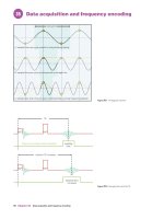
Data acquisition and frequency encoding 70
Data acquisition and phase encoding 72
Data acquisition and scan time 74
K space traversal and pulse sequences 76
Alternative K-space filling techniques 78
Signal to noise ratio 80
Contrast to noise ratio 82
Spatial resolution 84
Scan time 86
Trade-offs 87
Chemical shift 88
Out-of-phase artefact 90
Magnetic susceptibility 92
Phase wrap/aliasing 94
Phase mismapping (motion artefact) 96
Flow phenomena 98
Time-of-flight MR angiography 100

Phase contrast MR angiography 102
Contrast enhanced MR angiography 104
Contrast media 106
Magnets 108
Gradients 110
Radiofrequency coils 112
Other hardware 114
Bioeffects 116
Projectiles 118
Screening and safety procedures 120
Emergencies in the MR environment 121
Appendix 1 123
Appendix 2 124
Glossary 125
Index 129

iii


Preface
MRI at Glance is one of a series of books that presents complex
information in an easily accessible format. This series has become
famous for its concise text and clear diagrams. Since the first edition
of MRI at a Glance was published, the series has been updated to
include colour diagrams and a new layout with text on one page and
diagrams relating to the text on the opposite page. In this way all the
information on a particular topic is summarized so that the reader has
the essential points at their fingertips.
The second edition has been updated to reflect the new layout of the
series as a whole. Colour diagrams are now included and I have updated

the text to incorporate more detail on topics such as K space (which now
includes the famous Chest of Drawers analogy) and other developments like parallel imaging, EPI and diffusion. Each topic is presented

iv

on two pages for easy reference and large subjects have been broken
down into smaller sections. I have included simple explanations, analogies, bulleted lists, tables and plenty of images to aid the understanding
of each topic. There are also appendices on acronyms, abbreviations
and artefacts. The glossary has also been significantly expanded.
This book is intended to provide a concise overview of essential facts
for revision purposes and for those very new to MRI. For more detailed
explanations the reader is directed to MRI in Practice and Handbook of
MRI Technique. Indeed the diagrams and images in this book are taken
from these other texts and MRI at a Glance is intended to compliment
them.
I hope that everyone enjoys the new format. Happy Learning!


Acknowledgements
Once again I thank my friend and colleague John Talbot for his beautiful diagrams and for his support. We make a great team and long may it
continue! I also would like to thank Philips Medical Systems, Bill

Faulkner and Mike Kean for the use of some of their images in this
book. Thanks again to all my friends and family and especially to Toni,
Adam, Ben and Madeleine and to family in the USA.

Dedication
This book is dedicated to my ‘Dear Old Dad’, Joe Barbieri.

v

1
homogeneous
magnetic field

Magnetism and electromagnetism
paramagnetic
substance

paramagnetic substance
in the magnetic field
magnetic
field in
direction
of fingers

current in direction
of thumb

Figure 1.1 Paramagnetic properties.
conductor

homogeneous
magnetic field

diamagnetic
substance

diamagnetic substance
in the magnetic field

Figure 1.4 The right-hand thumb rule.

Figure 1.2 Diamagnetic properties.

homogeneous
magnetic field

ferromagnetic
substance

ferromagnetic substance
in the magnetic field

Figure 1.3 Ferromagnetic properties.

B0

Figure 1.5 A simple electromagnet.

2

Chapter 1 Magnetism and electromagnetism


Magnetic susceptibility
The magnetic susceptibility of a substance is the ability of external
magnetic fields to affect the nuclei of a particular atom, and is related to

the electron configurations of that atom. The nucleus of an atom, which
is surrounded by paired electrons, is more protected from, and unaffected by, the external magnetic field than the nucleus of an atom with
unpaired electrons. There are three types of magnetic susceptibility:
paramagnetism, diamagnetism and ferromagnetism.

(Figure 1.3). They are called magnetic lines of flux. The number of
lines per unit area is called the magnetic flux density. The strength
of the magnetic field, expressed by the notation (B) – or, in the case of
more than one field, the primary field (B0 ) and the secondary field (B1)
– is measured in one of three units: gauss (G), kilogauss (kG) and tesla
(T). If two magnets are brought close together, there are forces of attraction and repulsion between them depending on the orientation of their
poles relative to each other. Like poles repel and opposite poles attract.

Paramagnetism

Electromagnetism

Paramagnetic substances contain unpaired electrons within the atom
that induce a small magnetic field about themselves known as the
magnetic moment. With no external magnetic field these magnetic
moments occur in a random pattern and cancel each other out. In the
presence of an external magnetic field, paramagnetic substances align
with the direction of the field and so the magnetic moments add
together. Paramagnetic substances affect external magnetic fields
in a positive way, resulting in a local increase in the magnetic field
(Figure 1.1). An example of a paramagnetic substance is oxygen.

Magnetic fields are generated by moving charges (electrical current).
The direction of the magnetic field can either be clockwise or counterclockwise with respect to the direction of flow of the current. Ampere’s
law or Fleming’s right-hand rule determines the magnitude and direction of the magnetic field due to a current; if you point your right thumb

along the direction of the current, then the magnetic field points along
the direction of the curled fingers (Figure 1.4).
Just as moving electrical charge generates magnetic fields, changing
magnetic fields generate electric currents. When a magnet is moved in
and out of a closed circuit, an oscillating current is produced which
ceases the moment the magnet stops moving. Such a current is called an
induced electric current (Figure 1.5).
Faraday’s law of induction explains the phenomenon of an induced
current. The change of magnetic flux through a closed circuit induces an
electromotive force (emf ) in the circuit. The emf drives a current in the
circuit and is the result of a changing magnetic field inducing an electric
field.
The laws of electromagnetic induction (Faraday) state that the
induced emf:
(1) is proportional to the rate of change of magnetic field and the area
of the circuit;
(2) is in a direction so that it opposes the change in magnetic field
which causes it (Lenz’s law).
Electromagnetic induction is a basic physical phenomenon of MRI
but is specifically involved in the following:
• the spinning charge of a hydrogen proton causes a magnetic field to
be induced around it (see Chapter 2).
• the movement of the net magnetization vector (NMV) across the
area of a receiver coil induces an electrical charge in the coil (see
Chapter 4).

Diamagnetism
With no external magnetic field present, diamagnetic substances show
no net magnetic moment as the electron currents caused by their
motions add to zero.

When an external magnetic field is applied, diamagnetic substances
show a small magnetic moment that opposes the applied field. Substances of this type are therefore slightly repelled by the magnetic field
and have negative magnetic susceptibilities (Figure 1.2). Examples of
diamagnetic substances include water and inert gasses.

Ferromagnetism
When a ferromagnetic substance comes into contact with a magnetic
field, the results are strong attraction and alignment. They retain
their magnetization even when the external magnetic field has been
removed. Ferromagnetic substances remain magnetic, are permanently
magnetized and subsequently become permanent magnets. An example
of a ferromagnetic substance is iron.
Magnets are bipolar as they have two poles, north and south. The
magnetic field exerted by them produces magnetic field lines or lines of
force running from the magnetic south to the north poles of the magnet

Magnetism and electromagnetism Chapter 1 3


2

Atomic structure

magnetic moment

N

proton (positive)

neutron (no charge)

S
spin

electron (negative)

bar magnet

spin

spin

spin

orbit
direction

size

net spin

magnetic vector
Figure 2.2 The magnetic moment
of the hydrogen1 nucleus.

Figure 2.1 The atom.

4

Chapter 2 Atomic structure

Introduction

MR active nuclei

The atom consists of the following particles:
Protons
• in the nucleus
• are positively charged
Neutrons
• in the nucleus
• have no charge
Electrons
• orbit the nucleus
• are negatively charged (Figure 2.1).
The following terms are used to characterize an atom:
Atomic number: number of protons in the nucleus and determines the
type of element the atoms make up.
Mass number: sum of the neutrons and protons in the nucleus.
Atoms of the same element having a different mass number are called
isotopes.
In a stable atom the number of negatively charged electrons equals
the number of positively charged protons. Atoms with a deficit or excess
number of electrons are called ions.

Protons and neutrons spin about their own axis within the nucleus. The
direction of spin is random so that some particles spin clockwise, and
others anticlockwise.
When a nucleus has an even mass number the spins cancel each

other out so the nucleus has no net spin.
When a nucleus has an odd mass number, the spins do not cancel
each other out and the nucleus spins.
As protons have charge, a nucleus with an odd mass number has a net
charge as well as a net spin. Due to the laws of electromagnetic induction (see Chapter 1), a moving unbalanced charge induces a magnetic
field around itself. The direction and size of the magnetic field is
denoted by a magnetic moment or arrow (Figure 2.2). The total magnetic
moment of the nucleus is the vector sum of all the magnetic moments
of protons in the nucleus. The length of the arrow represents the magnitude of the magnetic moment. The direction of the arrow denotes the
direction of alignment of the magnetic moment.
Nuclei with an odd number of protons are said to be MR active. They
act like tiny bar magnets. There are many types of elements that are MR
active. They all have an odd mass number. The common MR active
nuclei, together with their mass numbers, are:
hydrogen 1 carbon 13 nitrogen
15 oxygen 17
fluorine 19 sodium 23 phosphorus 31
The isotope of hydrogen called protium is the MR active nucleus
used in MRI as it has a mass and atomic number of 1. The nucleus of this
isotope consists of a single proton and has no neutrons. It is used for MR
imaging because:
• it is abundant in the human body (e.g. in fat and water);
• its solitary proton gives it a relatively large magnetic moment.

Motion within the atom
• Negatively charged electrons spinning on their own axis.
• Negatively charged electrons orbiting the nucleus.
• Particles within the nucleus spinning on their own axes (Figure 2.1).
Each type of motion produces a magnetic field (see Chapter 1). In
MR we are concerned with the motion of particles within the nucleus

and the nucleus itself.

Atomic structure

Chapter 2 5


3

Alignment and precession
precessional path

precession
B0

B0
magnetic moment
of the nucleus

random alignment
no external field

alignment
external magnetic field

Figure 3.1 Alignment: classical theory.

low-energy spin-up nucleus

spinning

hydrogen
nucleus

low-energy spin-up population

Figure 3.3 Precession.

B0

B0
energy difference
depends upon field strength

high-energy spin-down nucleus

high-energy spin-down population

Figure 3.2 Alignment: quantum theory.

out of phase

in phase
Figure 3.4 Coherent and incoherent phase positions.
6

Chapter 3 Alignment and precession


Alignment
In a normal environment the magnetic moments of MR active nuclei

point in a random direction, and produce no overall magnetic effect.
When nuclei are placed in an external magnetic field their magnetic
moments line up with the magnetic field flux lines. This is called
alignment. Alignment is described using two theories.

The classical theory (Figure 3.1)
This uses the direction of the magnetic moments to illustrate alignment.
• Parallel alignment: alignment of magnetic moments in the same
direction as the main field.
• Anti-parallel alignment: alignment of magnetic moments in the
opposite direction to the main field.
At room temperature there are always more nuclei with their magnetic moments aligned parallel than anti-parallel. The net magnetism of
the patient (termed the net magnetization vector; NMV) is therefore
aligned parallel to the main field.
The quantum theory (Figure 3.2)
This uses the energy level of the nuclei to illustrate alignment. According to the quantum theory, magnetic moments of hydrogen nuclei align
in the presence of an external magnetic field in two energy states.
• Spin-up nuclei have low energy and do not have enough energy to
oppose the main field. These are nuclei that align their magnetic moments
parallel to the main field in the classical description.
• Spin-down nuclei have high energy and have enough energy to
oppose the main field. These are nuclei that align their magnetic moments
anti-parallel to the main field in the classical description.
The magnetic moments of the nuclei actually align at an angle to B0
due to the force of repulsion between B0 and the magnetic moments.
What do the quantum and classical theories tell us?
• Hydrogen only has two energy states – high or low. Therefore the
magnetic moments of hydrogen only align in the parallel or anti-parallel
directions. The magnetic moments of hydrogen cannot orientate
themselves in any other direction.

• The patient’s temperature is an important factor that determines whether
a nucleus is in the high or low energy population. In clinical imaging,
thermal effects are discounted as we assume the patient’s temperature is
the same inside and outside the magnetic field (thermal equilibrium).
• The magnetic moments of hydrogen are constantly changing their
orientation because nuclei are constantly moving between high and low
energy states. The nuclei gain and lose energy from B0 and their magnetic moments are constantly altering their alignment relative to B0.

• In thermal equilibrium, at any moment there are a greater proportion
of nuclei with their magnetic moments aligned with the field than
against it. This excess aligned with B0 produces a net magnetic effect
called the NMV that aligns with the main magnetic field.
• As the magnitude of the external magnetic field increases, more
magnetic moments line up in the parallel direction because the amount
of energy they must possess to oppose the stronger field and line up
anti-parallel is increased. As the field strength increases, the low-energy
population increases and the high-energy population decreases. As a
result the NMV increases.

Precession
Every MR active nucleus is spinning on its own axis. Due to the influence of the external magnetic field these nuclei produce a secondary
spin (Figure 3.3). This spin is called precession and causes the magnetic moments of MR active nuclei to describe a circular path around
B0. The speed at which the magnetic moments spin about the external
magnetic field is called the precessional frequency.
The Larmor equation is used to calculate the frequency or speed of
precession for a specific nucleus in a specific magnetic field strength.
The Larmor equation is stated as follows:
ω0 = B0 × λ
• The precessional frequency is denoted by ω0
• The strength of the external field is expressed in tesla (T) and denoted

by the symbol B0
• The gyromagnetic ratio is the precessional frequency of a specific
nucleus at 1T and has units of MHz/T. It is denoted by the Greek
symbol lambda (λ). As it is a constant of proportionality the precessional frequency is proportional to the strength of the external field.
The precessional frequencies of hydrogen (gyromagnetic ratio
42.57 MHz/T) commonly found in clinical MRI are:
• 21.285 MHz at 0.5 T
• 42.57 MHz at 1 T
• 63.86 MHz at 1.5 T
The precessional frequency corresponds to the range of frequencies
in the electromagnetic spectrum of radiowaves. Therefore hydrogen
precesses at a low frequency. At equilibrium the magnetic moments of
the nuclei are out of phase with each other. Phase refers to the position
of the magnetic moments on their precessional path.
• Out of phase or incoherent means that the magnetic moments of
hydrogen are at different places on the precessional path.
• In phase or coherent means that the magnetic moments of hydrogen
are at the same place on the precessional path (Figure 3.4).

Alignment and precession Chapter 3 7


4

Resonance and signal generation
low-energy population

some low-energy nuclei
gain enough energy to join
the high-energy population

B0

B0

flip angle

transverse plane

longitudinal plane

longitudinal plane

high-energy population

Figure 4.1 Energy transfer during excitation.

flip angle 90°

transverse plane

Figure 4.2 The flip angle. What flip angle gives maximum
transverse magnetization?

bore
B0
net
magnetic
vector

coil

precession

coil

top view
Figure 4.3 Generation of the MR signal. Why would you expect the MR signal to be alternating?
8

Chapter 4 Resonance and signal generation

end view


Resonance
Resonance is an energy transition that occurs when an object is subjected to a frequency the same as its own. In MR, resonance is induced
by applying a radiofrequency (RF) pulse:
• at the same frequency as the precessing hydrogen nuclei;
• at 90° to B0.
This causes the hydrogen nuclei to resonate (receive energy from the
RF pulse) whereas other types of MR active nuclei do not resonate. As
their gyromagnetic ratios are different from that of hydrogen their precessional frequencies are also different to that of hydrogen. They will
only resonate if RF at their specific precessional frequency is applied.
As RF is only applied at the same frequency as the precessional frequency of hydrogen, only hydrogen nuclei resonate. The other types of
MR active nuclei do not. Two things happen to the hydrogen nuclei at
resonance: energy absorption and phase coherence.

Energy absorption
The hydrogen nuclei absorb energy from the RF pulse (excitation
pulse). The absorption of applied RF energy at 90° to B0 causes an

increase in the number of high-energy, spin-down nuclei (Figure 4.1).
If just the right amount of energy is applied the number of nuclei in the
spin-up position equals the number in the spin-down position. As a
result the NMV (which represents the balance between spin-up and
spin-down nuclei) lies in a plane at 90° to the external field (the transverse plane) as the net magnetization lies between the two energy
states. As the NMV has been moved through 90° from B0, it has a flip
or tip angle of 90° (Figure 4.2).

Phase coherence

spin-up and spin-down positions and the spin-up nuclei are in phase
with the spin-down nuclei, the net effect is one of precession, so the
NMV precesses in the transverse plane at the Larmor frequency.

Learning point
It is important to understand that when a patient is placed in the magnet
and is scanned, hydrogen nuclei do not move. Nuclei are not flipped
onto their sides in the transverse plane and neither are their magnetic
moments. Only the magnetic moments of the nuclei move, aligning
either with or against B0. This is because hydrogen can only have
two energy states, high or low (see Chapter 3). It is the NMV that lies
in the transverse plane, not the magnetic moments, nor the nuclei
themselves.

The MR signal
A receiver coil is situated in the transverse plane. As the NMV rotates
around the transverse plane as a result of resonance, it passes across the
receiver coil inducing a voltage in it (see Chapter 1). This voltage is the
MR signal (Figure 4.3).
After a short period of time the RF pulse is removed. The signal

induced in the receiver coil begins to decrease. This is because the inphase component of the NMV in the transverse plane, which is passing
across the receiver coil, begins to decrease as an increasingly higher
proportion of spins become out of phase with each other. The amplitude
of the voltage induced in the receiver coil therefore decreases. This is
called free induction decay or FID:
• ‘free’ because of the absence of the RF pulse;
• ‘induction decay’ because of the decay of the induced signal in the
receiver coil.

The magnetic moments of the nuclei move into phase with each other
(see Chapter 3). As the magnetic moments are in phase both in the

Resonance and signal generation

Chapter 4 9


5

Contrast mechanisms

Figure 5.1 An axial image through the brain. Note the differences in contrast between CSF, fat, grey matter
and white matter.

TR

TR

RF
pulse

RF
pulse

RF
pulse

signal

TE

signal

TE

Figure 5.2 A basic pulse sequence showing TR and TE intervals.
10

Chapter 5 Contrast mechanisms


What is contrast?
An image has contrast if there are areas of high signal (white on the
image), as well as areas of low signal (dark on the image). Some areas
have an intermediate signal (shades of grey, between white and black).
The NMV can be separated into the individual vectors of the tissues
present in the patient such as fat, cerebrospinal fluid (CSF), grey matter
and white matter (Figure 5.1).
A tissue has a high signal (white, hyperintense) if it has a large
transverse component of magnetization when the signal is measured.

If there is a large component of transverse magnetization, the amplitude
of the magnetization that cuts the coil is large, and the signal induced in
the coil is also large.
A tissue has a low signal (black, hypointense), if it has a small
transverse component of magnetization when the signal is measured.
If there is a small component of transverse magnetization, the amplitude of the magnetization that cuts the coil is small, and the signal
induced in the coil is also small.
A tissue has an intermediate signal (grey, isointense), if it has a medium
transverse component of magnetization when the signal is measured.
Image contrast is controlled by extrinsic contrast parameters
(those that are controlled by the system operator). These include:
• Repetition time (TR): This is the time from the application of one
RF pulse to the application of the next for a particular slice. It is measured in milliseconds (ms). The TR affects the length of a relaxation
period in a particular slice after the application of one RF excitation
pulse to the beginning of the next (see Chapter 7) (Figure 5.2).
• Time to echo (TE): This is the time between an RF excitation pulse
and the collection of the signal. The TE affects the length of the relaxation period after the removal of an RF excitation pulse and the peak of
the signal received in the receiver coil (see Chapter 8). It is also measured in ms (Figure 5.2);

• Flip angle: This is the angle through which the NMV is moved as a
result of an RF excitation pulse (Figure 4.2);
• Turbo-factor (TF) or echo train length (ETL) (see Chapter 14);
• Time from inversion (TI) (see Chapter 16);
• ‘b’ value (see Chapter 25).
Image contrast is also controlled by intrinsic contrast mechanisms
(those that are inherent to the tissue and do not come under the
operator’s control). These include:
• T1 recovery time
• T2 decay time
• Proton density

• Flow
• Apparent diffusion coefficient (ADC).

The composition of fat and water
All substances possess molecules that are constantly in motion. This
molecular motion is made up of rotational and transitional movements
and is called Brownian motion. The faster the molecular motion, the
more difficult it is for a substance to release energy to its surroundings.
• Fat comprises hydrogen atoms mainly linked to carbon, that make up
large molecules. The large molecules in fat are closely packed together
and have a slow rate of molecular motion due to inertia of the large
molecules. They also have a low inherent energy which means they are
able to absorb energy efficiently.
• Water comprises hydrogen atoms linked to oxygen. It consists of
small molecules that are spaced far apart and have a high rate of molecular motion. They have a high inherent energy that means they are not
able to absorb energy efficiently.
Because of these differences, tissues that contain fat and water
produce different image contrast. This is because there are different
relaxation rates in each tissue.

Contrast mechanisms Chapter 5 11


6

Relaxation mechanisms
homogeneous

inhomogeneous

bore

bore

lower than centre frequency

centre frequency

higher than centre frequency

in phase

dephased

vector in area of lower field strength

vector in area of higher field strength

signal intensity

T2* curve

time

Figure 6.1 T2* decay and field inhomogeneities.
12

Chapter 6 Relaxation mechanisms

After the RF excitation pulse has been applied and resonance and
the desired flip angle achieved, the RF pulse is removed. The signal
induced in the receiver coil begins to decrease. This is because the
coherent component of NMV in the transverse plane, which is passing
across the receiver coil, begins to gradually decrease as an increasingly
higher proportion of spins become out of phase with each other. The
amplitude of the voltage induced in the receiver coil therefore gradually
decreases. This is called free induction decay or FID. The NMV in the
transverse plane decreases due to:
• relaxation processes;
• field inhomogeneities.

Relaxation processes
The magnetization in each tissue relaxes at different rates. This is one of
the factors that create image contrast.
The withdrawal of the RF produces several effects:
• Nuclei emit energy absorbed from the RF pulse through a process known as spin lattice energy transfer and shift their magnetic
moments from the high-energy state to the low-energy state. The
NMV recovers and realigns to B0. This relaxation process is called T1
recovery.
• Nuclei lose precessional coherence or dephase and the NMV decays
in the transverse plane. The dephasing relaxation process is called T2
decay.

Nuclei lose their coherence in two ways:
• by the interactions of the intrinsic magnetic fields of adjacent nuclei
(spin-spin) causing T2 decay (see Chapter 8);
• by inhomogeneities of the external magnetic field causing T2* decay.

Field inhomogeneities

Despite attempts to make the main magnetic field as uniform as
possible, inhomogeneities of the external magnetic field are inevitable
and slightly alter the magnitude of B0, i.e. some small areas of the field
have a magnetic field strength of slightly more or less than the main
field strength.
Due to the Larmor equation, the precessional frequency of a spin is
proportional to B0 (see Chapter 3). Spins that pass through these inhomogeneities experience magnetic field strengths that are slightly different from B0 and their precessional frequencies change. This results in a
change in their phase and dephasing of the NMV (Figure 6.1). Due to
a loss in phase coherence, transverse magnetization decays. This decay
occurs exponentially and is known as T2*. Magnetic field inhomogeneities cause the NMV to dephase before the intrinsic magnetic fields
of nuclei can influence dephasing, i.e. T2* happens before T2. In order
to produce images where T2 contrast can be visualized, ideally there
must be a mechanism to rephase spins and compensate for magnetic
field inhomogeneities. This is done by using pulse sequences (see
Chapter 12).

Relaxation mechanisms Chapter 6 13


T1 recovery
no contrast between
fat and water

7

contrast between
fat and water

63%

longitudinal
magnetization

longitudinal magnetization

100%

time
T1

time

short TR

long TR

Figure 7.2 T1 recovery in fat and water.
Figure 7.1 The T1 recovery curve.

first RF pulse

first RF pulse

B0

B0

transverse plane

transverse plane

transverse plane

second and succeeding
RF pulses

second and succeeding
RF pulses

B0

B0

B0

B0

B0

transverse plane

relaxation

B0

fat
water
transverse plane

water

fat
transverse plane

transverse plane

transverse plane

size of fat and water vectors
represent differences
in proton density

Figure 7.3 Saturation using a short TR.
14

Chapter 7 T1 recovery

Figure 7.4 Non-saturation using a long TR.


T1 recovery is caused by the exchange of energy from nuclei to their
surrounding environment or lattice. It is called spin lattice energy
transfer. As the nuclei dissipate their energy their magnetic moments
relax or return to B0, i.e. they regain their longitudinal magnetization.
The rate at which this occurs is an exponential process and occurs at
different rates in different tissues.
The T1 recovery time of a particular tissue is an intrinsic contrast
parameter that is inherent to the tissue being imaged. It is a constant
for a particular tissue and is defined as the time it takes for 63% of the
longitudinal magnetization to recover in that tissue (Figure 7.1). The

period of time during which this occurs is the time between one excitation pulse and the next or the TR (see Chapter 5). The TR therefore
determines how much T1 recovery occurs in a particular tissue.

T1 recovery in fat (Figure 7.2)
• T1 relaxation occurs as a result of nuclei exchanging the energy given
to them by the RF pulse to their surrounding environment. The efficiency of this process determines the T1 recovery time of the tissue in
which they are situated.
• Due to the fact that fat is able to absorb energy quickly (see Chapter 5),
the T1 recovery time of fat is very short, i.e. nuclei dispose of their
energy to the surrounding fat tissue and return to B0 in a short time.

T1 recovery in water (Figure 7.2)
• Water is very inefficient at receiving energy from nuclei (see Chapter 5).
The T1 recovery time of water is therefore quite long, i.e. nuclei take
a lot longer to dispose of their energy to the surrounding water tissue
and return to B0.
• In addition, the efficiency of spin lattice energy transfer depends on

how closely molecular motion of the molecules matches the Larmor
frequency. If there is a good match between the rate of molecular tumbling and the precessional frequency of spins, energy can be efficiently
exchanged between hydrogen and the surrounding molecular lattice.
• The Larmor frequency is relatively slow and therefore fat is much
better at this type of energy exchange than water, whose molecular
motion is much faster than the Larmor frequency (see Chapter 5). This
is another reason why fat has a shorter T1 recovery time than water.

Control of T1 recovery
The TR controls how much of the NMV in fat or water has recovered
before the application of the next RF pulse.
Short TRs do not permit full longitudinal recovery in most tissues

so that there are different longitudinal components in fat and water.
These different longitudinal components are converted to different
transverse components after the next excitation pulse has been applied.
As the NMV does not recover completely to the positive longitudinal
axis, they are pushed beyond the transverse plane by the succeeding 90°
RF pulse. This is called saturation. When saturation occurs there is a
contrast difference between fat and water due to differences in their T1
recovery times (Figure 7.3).
Long TRs allow full recovery of the longitudinal components in
most tissues. There is no difference in the magnitude of their longitudinal components. There is no contrast difference between fat and water
due to differences in T1 recovery times when using long TRs. Any differences seen in contrast are due to differences in the number of protons
or proton density of each tissue. The proton density of a particular
tissue is an intrinsic contrast parameter and is therefore inherent to the
tissue being imaged (Figure 7.4).

T1 recovery Chapter 7 15


T2 decay

transverse magnetization

8

water

fat
time

small amount of dephasing

=

large transverse
component of
magnetization

large amount of dephasing

=

small transverse
component of
magnetization
Figure 8.1 T2 contrast generation.

coherent transverse magnetization

100%

37%

T2

time
Figure 8.2 The T2 decay curve.

16

Chapter 8 T2 decay

large
contrast
difference
between
fat and water

coherent transverse magnetization

small
contrast
difference
between
fat and water

long T2 (water)
short T2 fat

time

short TE

long TE

T2 decay is caused by the interaction between the magnetic fields of
neighbouring spins. It is called spin-spin. It occurs as a result of the
intrinsic magnetic fields of the nuclei interacting with each other. This
produces a loss of phase coherence or dephasing, and results in decay of
the NMV in the transverse plane. It is an exponential process and occurs

at different rates in different tissues (Figure 8.1).
The T2 decay time of a particular tissue is an intrinsic contrast
parameter and is inherent to the tissue being imaged. It is the time it
takes for 63% of the transverse magnetization to be lost due to dephasing, i.e. transverse magnetization is reduced by 63% of its original value
(37% remains) (Figure 8.2). The period of time during which this
occurs is the time between the excitation pulse and the MR signal or the
TE (see Chapter 5). The TE therefore determines how much T2 decay
occurs in a particular tissue.

T2 decay in fat and water (Figure 8.3)
T2 relaxation occurs as a result of the spins of adjacent nuclei interacting

Figure 8.3 T2 decay in fat and water.

with each other and exchanging energy. The efficiency of this process
depends on how closely packed the molecules are to each other.
• In fat the molecules are more closely packed together than in water so
that spin-spin is more efficient (see Chapter 5). The T2 time of fat is
therefore very short compared to that of water.
• The TE controls how much transverse magnetization has been
allowed to decay in fat and water when the signal is read.
Short TEs do not permit full dephasing in either fat or water, so their
coherent transverse components are similar. There is little contrast difference between fat and water due to differences in T2 decay times
using short TEs.
Long TEs allow dephasing of the transverse components in fat and
water. There is a contrast difference between fat and water due to differences in T2 decay times when using long TEs.
It should be noted that fat and water represent the extremes in image
contrast. Other tissues, such as muscle, grey matter and white matter
have contrast characteristics that fall between fat and water.

T2 decay

Chapter 8 17


9

T1 weighting

Figure 9.1 Axial T1 weighted image of the brain.

Figure 9.2 Coronal T1 weighted image of the knee.

Figure 9.3 Sagittal T1 weighted image of the lumbar spine.

18

Chapter 9 T1 weighting