KINH TẾ VI MÔ 2015 chapter 4 (part 2) micro 1 5 producers choice
Bạn đang xem bản rút gọn của tài liệu. Xem và tải ngay bản đầy đủ của tài liệu tại đây (622.25 KB, 10 trang )
12/21/2015
Part 2- Contents
1. Production in the Long-run
Chapter 4
2. Cost in the Long –run
MICROECONOMICS
Theories of Producer
Behavior
By Tran ThiKieu Minh, MSc.
2015, FTU Kieu Minh
1
4.4. Production in the Long-run
2
Production:Two Variable Inputs
Two Variable Inputs
The information can be represented graphically
Firm can produce output by combining
using isoquants
different amounts of labor and capital
2015, FTU Kieu Minh
2015, FTU Kieu Minh
◦ Curves showing all possible combinations of inputs
that yield the same output
3
2015, FTU Kieu Minh
4
1
12/21/2015
Isoquant Map
Capital
per year
Production:Two Variable Inputs
E
5
4
3
A
B
C
2
q3 = 90
D
1
q2 = 75
Amount by which the quantity of one input can be reduced when
one extra unit of another input is used, so that output remains
constant.
q1 = 55
1
2
3
4
5
Labor per year
2015, FTU Kieu Minh
Substituting Among Inputs
◦ There is a trade-off between inputs allowing them to use
more of one input and less of another for the same level
of output.
◦ Slope of the isoquant shows how one input can be
substituted for the other and keep the level of output
the same.
◦ Positive slope is the marginal rate of technical
substitution (MRTS)
Ex: 55 units of output
can be produced with
3K & 1L (pt. A)
OR
1K & 3L (pt. D)
5
2015, FTU Kieu Minh
6
Marginal Rate of
Technical Substitution
Production:Two Variable Inputs
Capital
per year
The marginal rate of technical substitution
equals:
5
4
Changein Capital input
Changein Labor input
MRTS K
(for a fixed level of q )
L
MRTS
Slope measures MRTS
MRTS decreases as move down
the indifference curve
2
1
3
1
1
2
Q3 =90
2/3 1
1/3
1
Q2 =75
1
Q1 =55
1
2015, FTU Kieu Minh
7
2015, FTU Kieu Minh
2
3
4
5
Labor per month
8
2
12/21/2015
MRTS and Isoquants
Isoquants: Special Cases
Diminishing MRTS occurs because of diminishing returns
and implies isoquants are convex.
There is a relationship between MRTS and marginal
products of inputs. If we are holding output constant
2015, FTU Kieu Minh
Two extreme cases show the possible range of
input substitution in production
1. Perfect substitutes
9
B
C
2015, FTU Kieu Minh
10
Q2
Q3
Extreme cases (cont.)
2. Perfect Complements
◦ Fixed proportions production function
◦ There is no substitution available between inputs
◦ The output can be made with only a specific
proportion of capital and labor
◦ Cannot increase output unless increase both
capital and labor in that specific proportion
Same output can be
reached with mostly
capital or mostly labor (A
or C) or with equal
amount of both (B)
Q1
Same output can be produced with a lot of capital
or a lot of labor or a balanced mix
Isoquants: Special Cases
A
MRTS is constant at all points on isoquant
◦
2015, FTU Kieu Minh
Perfect Substitutes
Capital
per
month
◦
Labor
per month
11
2015, FTU Kieu Minh
12
3
12/21/2015
Fixed-Proportions
Production Function
4.5 Cost in the Long Run
Capital
per
month
Same output can only
be produced with one
set of inputs.
Q3
C
B
Q1
A
Labor
per month
2015, FTU Kieu Minh
Assumptions
◦ Two Inputs: Labor (L) & capital (K)
◦ Price of labor: wage rate (w)
◦ The price of capital
r = depreciation rate + interest rate
Or rental rate if not purchasing
These are equal in a competitive capital market
Q2
K1
In the long run a firm can change all of its inputs
In making cost minimizing choices, must look at the
cost of using capital and labor in production
decisions
L1
13
2015, FTU Kieu Minh
14
Isocost Line
Cost in the Long Run
Capital
per
year
Total cost of production
C = wL + rK
K2
or K = C/r - (w/r)L
The Isocost Line
r
◦ A line showing all combinations of L & K that can be
purchased for the same cost
Slope w
◦ For each different level of cost, the equation shows
another isocost line
A
K1
K3
C0
L2
2015, FTU Kieu Minh
15
2015, FTU Kieu Minh
L1
C1
L3
C2
Labor per year
16
4
12/21/2015
Producing a Given Output at
Minimum Cost
Choosing Inputs
We will address how to minimize cost for a
Capital
per
year
given level of output by combining isocosts with
isoquants
We choose the output we wish to produce and
then determine how to do that at minimum
cost
Q1 is an isoquant for output Q1.
There are three isocost lines, of
which 2 are possible choices in
which to produce Q1
K2
Isocost C2 shows quantity
Q1 can be produced with
combination K2L2 or K 3L3.
However, both of these
are higher cost combinations
than K 1L1.
A
◦ Isoquant is the quantity we wish to produce
◦ Isocost is the combination of K and L that gives a set
cost
K1
Q1
K3
C0
L2
2015, FTU Kieu Minh
17
The minimum cost combination can then be
written as:
production process?
L
MPL
Slope of isocost line K
2015, FTU Kieu Minh
MPK
w
r
18
Choosing Inputs
How does the isocost line relate to the firm’s
MPL
Labor per year
2015, FTU Kieu Minh
Choosing Inputs
MRTS - K
C2
C1
L3
L1
MPL
MPK
L
w
◦
r
w
MPK
r
Minimum cost for a given output will occur when
each dollar of input added to the production process
will add an equivalent amount of output.
when firmminimizes cost
19
2015, FTU Kieu Minh
20
5
12/21/2015
Ex
Quiz
If w = $10, r = $20, and MPL = MP K, which input
would be used more of?
MPL MPK
10 20
2015, FTU Kieu Minh
21
A firm operates with the production function Q = K 2 L. The
manager has been given a production target: Produce 8,000
units per day. She knows that the daily rental price of capital is
$400 per unit. The wage rate paid to each worker is $200 day.
a) Currently the firm employs at 80 workers per day. What is the
firm’s daily total cost if it rents just enough capital to produce
at its target?
b) Compare the marginal product per dollar sent on K and on L
when the firm operates at the input choice in part (a). What
does this suggest about the way the firm might change its
choice of K and L if it wants to reduce the total cost in
meeting its target?
c) In the long run, how much K and L should the firm choose if it
wants to minimize the cost of producing 8,000 units of output
day? What will the total daily cost of production be?
2015, FTU Kieu Minh
22
A Firm’s Expansion Path
Cost in the Long Run
Cost minimization with Varying Output Levels
Capital
per
year
◦ For each level of output, there is an isocost curve
showing minimum cost for that output level
◦ A firm’s expansion path shows the minimum cost
combinations of labor and capital at each level of
output.
The expansion path illustrates
the least-cost combinations of
labor and capital that can be
used to produce each level of
output in the long-run.
150 $3000
Expansion Path
$200
100 0
C
75
◦ Slope equals K/L
B
50
300 Units
A
25
200 Units
2015, FTU Kieu Minh
23
2015, FTU Kieu Minh
50
100
150
200
300
Labor per year
24
6
12/21/2015
A Firm’s Long-Run Total Cost
Curve
Expansion Path & Long-run Costs
Firms expansion path has same information as
Cost/
Year
long-run total cost curve
To move from expansion path to LR cost curve
Long Run Total Cost
F
3000
◦ Find tangency with isoquant and isocost
E
◦ Determine min cost of producing the output level
selected
◦ Graph output-cost combination
2000
D
1000
100
2015, FTU Kieu Minh
25
Long-Run Versus
Short-Run Cost Curves
If input is doubled, output will double
AC cost is constant at all levels of output.
2015, FTU Kieu Minh
Output, Units/yr
26
2. Increasing Returns to Scale
Most important determinant of the shape of the
LR AC and MC curves is relationship between
scale of the firm’s operation and inputs required to
min cost
1. Constant Returns to Scale
◦
◦
300
Long-Run Versus Short-Run Cost
Curves
Long-Run Average Cost (LAC)
◦
200
2015, FTU Kieu Minh
27
◦
◦
If input is doubled, output will more than double
AC decreases at all levels of output.
3. Decreasing Returns to Scale
◦
If input is doubled, output will less than double
◦
AC increases at all levels of output
2015, FTU Kieu Minh
28
7
12/21/2015
Long-Run Versus Short-Run Cost
Curves
Long-Run Versus Short-Run Cost
Curves
In the long-run:
◦ Firms experience increasing and decreasing returns
to scale and therefore long-run average cost is “U”
shaped.
◦ Source of U-shape is due to returns to scale rather
than diminishing marginal returns to a factor of
production
◦ Long-run marginal cost curve measures the change in
long-run total costs as output is increased by 1 unit
Long-run marginal cost leads long-run
average cost:
◦ If LMC < LAC, LAC will fall
◦ If LMC > LAC, LAC will rise
◦ Therefore, LMC = LAC at the minimum of
LAC
In special case where LAC if constant,
LAC and LMC are equal
2015, FTU Kieu Minh
29
2015, FTU Kieu Minh
Long-Run Average and Marginal
Cost
Long Run Costs
Cost
($ per unit
of output
30
LMC
As output increases, firm’s AC of producing is
likely to decline to a point
1. On a larger scale, workers can better specialize
2. Scale can provide flexibility – managers can
organize production more effectively
LAC
A
3. Firm may be able to get inputs at lower cost if it
can get quantity discounts. Lower prices might
lead to different input mix
Output
2015, FTU Kieu Minh
31
2015, FTU Kieu Minh
32
8
12/21/2015
Long Run Costs
Long Run Costs
At some point, AC will begin to increase
When input proportions change, the firm’s
1. Factory space and machinery may make it more
difficult for workers to do their job efficiently
2. Managing a larger firm may become more complex
and inefficient as the number of tasks increase
3. Bulk discounts can no longer be utilized. Limited
availability of inputs may cause price to rise
Economies of scale reflects input proportions
2015, FTU Kieu Minh
expansion path is no longer a straight line
◦ Concept of return to scale no longer applies
that change as the firm change its level of
production
Unlike returns to scale, economies of scale
allows inputs proportions vary
33
Economies and Diseconomies of
Scale
34
Quiz
Economies of Scale
◦ Increase in output is greater than the increase in
inputs.
Diseconomies of Scale
◦ Increase in output is less than the increase in inputs.
U-shaped LAC shows economies of scale for
relatively low output levels and diseconomies of
scale for higher levels
2015, FTU Kieu Minh
2015, FTU Kieu Minh
35
In the long run for Firm A, total cost is $105 when
output is 3 units and $120 when output is 4 units.
Does Firm A exhibit economies or diseconomies of
scale?
a. Diseconomies of scale, since total cost is rising as
output rises.
b. Diseconomies of scale, since average total cost is
falling as output rises.
c. Economies of scale, since total cost is rising as output
rises.
d. Economies of scale, since average total cost is falling
as output rises.
2015, FTU Kieu Minh
36
9
12/21/2015
Long-Run Versus Short-Run Cost
Curves
Average total cost in the short and long runs
Average
Total
Cost
We will use short and long-run cost to
ATC in short ATC in short
run with
run with
small factory medium factory
ATC in short
run with
large factory
LAC
determine the optimal plant size
We can show the short run average costs for 3
different plant sizes
This decision is important because once built,
$12,000
the firm may not be able to change plant size
for a while
10,000
Economies
of scale
Constant returns to scale
Diseconomies
of scale
0
1,000 1,200
Quantity of Cars per Day
Because fixed costs are variable in the long run, the average-total-cost curve in the short run differs
from the average-total-cost curve in the long run.
2015, FTU Kieu Minh
37
2015, FTU Kieu Minh
38
Average total cost in the short and long
runs
Firm will always choose plant that minimizes the
average cost of production
The long-run average cost curve envelopes the
short-run average cost curves
The LAC curve exhibits economies of scale
initially but exhibits diseconomies at higher
output levels
2015, FTU Kieu Minh
The firm experiences diseconomies of scale if it changes its
level of output
a. from Q1 to Q2.
b. from Q2 to Q3.
c. from Q3 to Q4.
d. from Q4 to Q5.
39
2015, FTU Kieu Minh
40
10