Blahut r e fast algorithms for signal Processin(BookZZ org)
Bạn đang xem bản rút gọn của tài liệu. Xem và tải ngay bản đầy đủ của tài liệu tại đây (1.98 MB, 469 trang )
This page intentionally left blank
Fast Algorithms for Signal Processing
Efficient algorithms for signal processing are critical to very large scale future applications such as video processing and four-dimensional medical imaging. Similarly,
efficient algorithms are important for embedded and power-limited applications since,
by reducing the number of computations, power consumption can be reduced considerably. This unique textbook presents a broad range of computationally-efficient
algorithms, describes their structure and implementation, and compares their relative
strengths. All the necessary background mathematics is presented, and theorems are
rigorously proved. The book is suitable for researchers and practitioners in electrical
engineering, applied mathematics, and computer science.
Richard E. Blahut is a Professor of Electrical and Computer Engineering at the University
of Illinois, Urbana-Champaign. He is Life Fellow of the IEEE and the recipient of
many awards including the IEEE Alexander Graham Bell Medal (1998) and Claude E.
Shannon Award (2005), the Tau Beta Pi Daniel C. Drucker Eminent Faculty Award,
and the IEEE Millennium Medal. He was named a Fellow of the IBM Corporation in
1980, where he worked for over 30 years, and was elected to the National Academy of
Engineering in 1990.
Fast Algorithms for
Signal Processing
Richard E. Blahut
Henry Magnuski Professor in Electrical and Computer Engineering,
University of Illinois, Urbana-Champaign
CAMBRIDGE UNIVERSITY PRESS
Cambridge, New York, Melbourne, Madrid, Cape Town, Singapore,
São Paulo, Delhi, Dubai, Tokyo
Cambridge University Press
The Edinburgh Building, Cambridge CB2 8RU, UK
Published in the United States of America by Cambridge University Press, New York
www.cambridge.org
Information on this title: www.cambridge.org/9780521190497
© Cambridge University Press 2010
This publication is in copyright. Subject to statutory exception and to the
provision of relevant collective licensing agreements, no reproduction of any part
may take place without the written permission of Cambridge University Press.
First published in print format 2010
ISBN-13
978-0-511-77637-3
eBook (NetLibrary)
ISBN-13
978-0-521-19049-7
Hardback
Cambridge University Press has no responsibility for the persistence or accuracy
of urls for external or third-party internet websites referred to in this publication,
and does not guarantee that any content on such websites is, or will remain,
accurate or appropriate.
In loving memory of
Jeffrey Paul Blahut
May 2, 1968 – June 13, 2004
Many small make a great.
— Chaucer
Contents
Preface
Acknowledgments
1
Introduction
1.1
1.2
1.3
1.4
1.5
2
3
vii
Introduction to fast algorithms
Applications of fast algorithms
Number systems for computation
Digital signal processing
History of fast signal-processing algorithms
xi
xiii
1
1
6
8
9
17
Introduction to abstract algebra
21
2.1
2.2
2.3
2.4
2.5
2.6
2.7
2.8
21
26
30
34
37
44
48
58
Groups
Rings
Fields
Vector space
Matrix algebra
The integer ring
Polynomial rings
The Chinese remainder theorem
Fast algorithms for the discrete Fourier transform
68
3.1
3.2
3.3
68
72
80
The Cooley–Tukey fast Fourier transform
Small-radix Cooley–Tukey algorithms
The Good–Thomas fast Fourier transform
viii
Contents
3.4
3.5
3.6
3.7
3.8
4
5
6
The Goertzel algorithm
The discrete cosine transform
Fourier transforms computed by using convolutions
The Rader–Winograd algorithm
The Winograd small fast Fourier transform
83
85
91
97
102
Fast algorithms based on doubling strategies
115
4.1
4.2
4.3
4.4
4.5
4.6
4.7
4.8
115
119
120
122
124
127
130
139
Halving and doubling strategies
Data structures
Fast algorithms for sorting
Fast transposition
Matrix multiplication
Computation of trigonometric functions
An accelerated euclidean algorithm for polynomials
A recursive radix-two fast Fourier transform
Fast algorithms for short convolutions
145
5.1
5.2
5.3
5.4
5.5
5.6
5.7
5.8
145
148
155
164
168
171
176
178
Cyclic convolution and linear convolution
The Cook–Toom algorithm
Winograd short convolution algorithms
Design of short linear convolution algorithms
Polynomial products modulo a polynomial
Design of short cyclic convolution algorithms
Convolution in general fields and rings
Complexity of convolution algorithms
Architecture of filters and transforms
194
6.1
6.2
6.3
6.4
6.5
6.6
6.7
6.8
194
199
202
207
213
216
221
222
Convolution by sections
Algorithms for short filter sections
Iterated filter sections
Symmetric and skew-symmetric filters
Decimating and interpolating filters
Construction of transform computers
Limited-range Fourier transforms
Autocorrelation and crosscorrelation
ix
Contents
7
Fast algorithms for solving Toeplitz systems
231
7.1
7.2
7.3
7.4
7.5
231
239
245
249
255
8
9
10
The Levinson and Durbin algorithms
The Trench algorithm
Methods based on the euclidean algorithm
The Berlekamp–Massey algorithm
An accelerated Berlekamp–Massey algorithm
Fast algorithms for trellis search
262
8.1
8.2
8.3
8.4
8.5
8.6
262
267
270
274
278
280
Trellis and tree searching
The Viterbi algorithm
Sequential algorithms
The Fano algorithm
The stack algorithm
The Bahl algorithm
Numbers and fields
286
9.1
9.2
9.3
9.4
9.5
9.6
9.7
286
293
296
299
300
304
306
Elementary number theory
Fields based on the integer ring
Fields based on polynomial rings
Minimal polynomials and conjugates
Cyclotomic polynomials
Primitive elements
Algebraic integers
Computation in finite fields and rings
311
10.1
10.2
10.3
10.4
10.5
10.6
10.7
311
314
317
320
324
328
331
Convolution in surrogate fields
Fermat number transforms
Mersenne number transforms
Arithmetic in a modular integer ring
Convolution algorithms in finite fields
Fourier transform algorithms in finite fields
Complex convolution in surrogate fields
x
11
12
Contents
10.8 Integer ring transforms
10.9 Chevillat number transforms
10.10 The Preparata–Sarwate algorithm
336
339
339
Fast algorithms and multidimensional convolutions
345
11.1
11.2
11.3
11.4
11.5
11.6
11.7
11.8
345
350
357
362
368
371
372
376
Nested convolution algorithms
The Agarwal–Cooley convolution algorithm
Splitting algorithms
Iterated algorithms
Polynomial representation of extension fields
Convolution with polynomial transforms
The Nussbaumer polynomial transforms
Fast convolution of polynomials
Fast algorithms and multidimensional transforms
384
12.1
12.2
12.3
12.4
12.5
12.6
12.7
12.8
384
389
391
395
399
403
410
411
Small-radix Cooley–Tukey algorithms
The two-dimensional discrete cosine transform
Nested transform algorithms
The Winograd large fast Fourier transform
The Johnson–Burrus fast Fourier transform
Splitting algorithms
An improved Winograd fast Fourier transform
The Nussbaumer–Quandalle permutation algorithm
A
A collection of cyclic convolution algorithms
427
B
A collection of Winograd small FFT algorithms
435
Bibliography
Index
442
449
Preface
A quarter of a century has passed since the previous version1 of this book was published,
and signal processing continues to be a very important part of electrical engineering.
It forms an essential part of systems for telecommunications, radar and sonar, image
formation systems such as medical imaging, and other large computational problems,
such as in electromagnetics or fluid dynamics, geophysical exploration, and so on. Fast
computational algorithms are necessary in large problems of signal processing, and
the study of such algorithms is the subject of this book. Over those several decades,
however, the nature of the need for fast algorithms has shifted both to much larger
systems on the one hand and to embedded power-limited applications on the other.
Because many processors and many problems are much larger now than they were
when the original version of this book was written, and the relative cost of addition and
multiplication now may appear to be less dramatic, some of the topics of twenty years
ago may be seen by some to be of less importance today. I take exactly the opposite
point of view for several reasons. Very large three-dimensional or four-dimensional
problems now under consideration require massive amounts of computation and this
computation can be reduced by orders of magnitude in many cases by the choice
of algorithm. Indeed, these very large problems can be especially suitable for the
benefits of fast algorithms. At the same time, smaller signal processing problems now
appear frequently in handheld or remote applications where power may be scarce
or nonrenewable. The designer’s care in treating an embedded application, such as
a digital television, can repay itself many times by significantly reducing the power
expenditure. Moreover, the unfamiliar algorithms of this book now can often be handled
automatically by computerized design tools, and in embedded applications where power
dissipation must be minimized, a search for the algorithm with the fewest operations
may be essential.
Because the book has changed in its details and the title has been slightly modernized,
it is more than a second edition, although most of the topics of the original book have
been retained in nearly the same form, but usually with the presentation rewritten.
Possibly, in time, some of these topics will re-emerge in a new form, but that time
1
xi
Fast Algorithms for Digital Signal Processing, Addison-Wesley, Reading, MA, 1985.
xii
Preface
is not now. A newly written book might look different in its choice of topics and
its balance between topics than does this one. To accommodate this consideration
here, the chapters have been rearranged and revised, even those whose content has not
changed substantially. Some new sections have been added, and all of the book has
been polished, revised, and re-edited. Most of the touch and feel of the original book
is still evident in this new version.
The heart of the book is in the Fourier transform algorithms of Chapters 3 and 12
and the convolution algorithms of Chapters 5 and 11. Chapters 12 and 11 are the multidimensional continuations of Chapters 3 and 4, respectively, and can be partially read
immediately thereafter if desired. The study of one-dimensional convolution algorithms
and Fourier transform algorithms is only completed in the context of the multidimensional problems. Chapters 2 and 9 are mathematical interludes; some readers may
prefer to treat them as appendices, consulting them only as needed. The remainder,
Chapters 4, 7, and 8, are in large part independent of the rest of the book. Each can be
read independently with little difficulty.
This book uses branches of mathematics that the typical reader with an engineering
education will not know. Therefore these topics are developed in Chapters 2 and 9, and
all theorems are rigorously proved. I believe that if the subject is to continue to mature
and stand on its own, the necessary mathematics must be a part of such a book; appeal
to a distant authority will not do. Engineers cannot confidently advance through the
subject if they are frequently asked to accept an assertion or to visit their mathematics
library.
Acknowledgments
My major debt in writing this book is to Shmuel Winograd. Without his many contributions to the subject, the book would be shapeless and much shorter. He was also
generous with his time in clarifying many points to me, and in reviewing early drafts
of the original book. The papers of Winograd and also the book of Nussbaumer were
a source for much of the material discussed in this book.
The original version of this book could not have reached maturity without being
tested, critiqued, and rewritten repeatedly. I remain indebted to Professor B. W.
Dickinson, Professor Toby Berger, Professor C. S. Burrus, Professor J. Gibson, Professor J. G. Proakis, Professor T. W. Parks, Dr B. Rice, Professor Y. Sugiyama,
Dr W. Vanderkulk, and Professor G. Verghese for their gracious criticisms of the
original 1985 manuscript. That book could not have been written without the support
that was given by the International Business Machines Corporation. I am deeply grateful to IBM for this support and also to Cornell University for giving me the opportunity
to teach several times from the preliminary manuscript of the earlier book. The revised
book was written in the wonderful collaborative environment of the Department of
Electrical and Computer Engineering and the Coordinated Science Laboratory of the
University of Illinois. The quality of the book has much to with the composition skills
of Mrs Francie Bridges and the editing skills of Mrs Helen Metzinger. And, as always,
Barbara made it possible.
xiii
1
Introduction
Algorithms for computation are found everywhere, and efficient versions of these
algorithms are highly valued by those who use them. We are mainly concerned with
certain types of computation, primarily those related to signal processing, including
the computations found in digital filters, discrete Fourier transforms, correlations, and
spectral analysis. Our purpose is to present the advanced techniques for fast digital
implementation of these computations. We are not concerned with the function of a
digital filter or with how it should be designed to perform a certain task; our concern is
only with the computational organization of its implementation. Nor are we concerned
with why one should want to compute, for example, a discrete Fourier transform;
our concern is only with how it can be computed efficiently. Surprisingly, there is
an extensive body of theory dealing with this specialized topic – the topic of fast
algorithms.
1.1
Introduction to fast algorithms
An algorithm, like most other engineering devices, can be described either by an
input/output relationship or by a detailed explanation of its internal construction. When
one applies the techniques of signal processing to a new problem one is concerned only
with the input/output aspects of the algorithm. Given a signal, or a data record of some
kind, one is concerned with what should be done to this data, that is, with what the
output of the algorithm should be when such and such a data record is the input. Perhaps
the output is a filtered version of the input, or the output is the Fourier transform of the
input. The relationship between the input and the output of a computational task can
be expressed mathematically without prescribing in detail all of the steps by which the
calculation is to be performed.
Devising such an algorithm for an information processing problem, from this
input/output point of view, may be a formidable and sophisticated task, but this is
not our concern in this book. We will assume that we are given a specification of a
relationship between input and output, described in terms of filters, Fourier transforms,
interpolations, decimations, correlations, modulations, histograms, matrix operations,
1
2
Introduction
and so forth. All of these can be expressed with mathematical formulas and so can be
computed just as written. This will be referred to as the obvious implementation.
One may be content with the obvious implementation, and it might not be apparent
that the obvious implementation need not be the most efficient. But once people began
to compute such things, other people began to look for more efficient ways to compute
them. This is the story we aim to tell, the story of fast algorithms for signal processing.
By a fast algorithm, we mean a detailed description of a computational procedure
that is not the obvious way to compute the required output from the input. A fast
algorithm usually gives up a conceptually clear computation in favor of one that is
computationally efficient.
Suppose we need to compute a number A, given by
A = ac + ad + bc + bd.
As written, this requires four multiplications and three additions to compute. If we
need to compute A many times with different sets of data, we will quickly notice that
A = (a + b)(c + d)
is an equivalent form that requires only one multiplication and two additions, and so
it is to be preferred. This simple example is quite obvious, but really illustrates most
of what we shall talk about. Everything we do can be thought of in terms of the clever
insertion of parentheses in a computational problem. But in a big problem, the fast
algorithms cannot be found by inspection. It will require a considerable amount of
theory to find them.
A nontrivial yet simple example of a fast algorithm is an algorithm for complex
multiplication. The complex product1
(e + jf ) = (a + jb) · (c + jd)
can be defined in terms of real multiplications and real additions as
e = ac − bd
f = ad + bc.
We see that these formulas require four real multiplications and two real additions.
A more efficient “algorithm” is
e = (a − b)d + a(c − d)
f = (a − b)d + b(c + d)
whenever multiplication is harder than addition. This form requires three real multiplications and five real additions. If c and d are constants for a series of complex
1
The letter j is used for
√
−1 and j is used as an index throughout the book. This should not cause any confusion.
3
1.1 Introduction to fast algorithms
multiplications, then the terms c + d and c − d are constants also and can be computed
off-line. It then requires three real multiplications and three real additions to do one
complex multiplication.
We have traded one multiplication for an addition. This can be a worthwhile saving,
but only if the signal processor is designed to take advantage of it. Most signal processors, however, have been designed with a prejudice for a complex multiplication
that uses four multiplications. Then the advantage of the improved algorithm has no
value. The storage and movement of data between additions and multiplications are
also important considerations in determining the speed of a computation and of some
importance in determining power dissipation.
We can dwell further on this example as a foretaste of things to come. The complex
multiplication above can be rewritten as a matrix product
e
f
=
c
d
−d
c
where the vector
a
,
b
c
a
represents the complex number a + jb, the matrix
d
b
−d
c
e
represents the complex
f
number e + jf . The matrix–vector product is an unconventional way to represent
complex multiplication. The alternative computational algorithm can be written in
matrix form as
1
0
(c − d)
0
0
1 0 1
e
a
.
=
1
(c + d) 0 0
0
b
0 1 1
f
1 −1
0
0
d
represents the complex number c + jd, and the vector
The algorithm, then, can be thought of as nothing more than the unusual matrix
factorization:
1
0
(c − d)
0
0
1 0 1
c −d
=
1 .
(c + d) 0 0
0
0 1 1
d
c
1 −1
0
0
d
We can abbreviate the algorithm as
e
a
= BDA
,
f
b
where A is a three by two matrix that we call a matrix of preadditions; D is a three by
three diagonal matrix that is responsible for all of the general multiplications; and B is
a two by three matrix that we call a matrix of postadditions.
4
Introduction
We shall find that many fast computational procedures for convolution and for the
discrete Fourier transform can be put into this factored form of a diagonal matrix in
the center, and on each side of which is a matrix whose elements are 1, 0, and −1.
Multiplication by a matrix whose elements are 0 and ±1 requires only additions and
subtractions. Fast algorithms in this form will have the structure of a batch of additions,
followed by a batch of multiplications, followed by another batch of additions.
The final example of this introductory section is a fast algorithm for multiplying two
arbitrary matrices. Let
C = AB,
where A and B are any by n, and n by m, matrices, respectively. The standard method
for computing the matrix C is
n
cij =
aik bkj
k=1
i = 1, . . . ,
j = 1, . . . , m,
which, as it is written, requires m n multiplications and (n − 1) m additions. We shall
give an algorithm that reduces the number of multiplications by almost a factor of
two but increases the number of additions. The total number of operations increases
slightly.
We use the identity
a1 b1 + a2 b2 = (a1 + b2 )(a2 + b1 ) − a1 a2 − b1 b2
on the elements of A and B. Suppose that n is even (otherwise append a column of
zeros to A and a row of zeros to B, which does not change the product C). Apply the
above identity to pairs of columns of A and pairs of rows of B to write
n/2
cij =
(ai,2k−1 b2k−1,j + ai,2k b2k,j )
i=1
n/2
=
n/2
(ai,2k−1 + b2k,j )(ai,2k + b2k−1,j ) −
k=1
n/2
ai,2k−1 ai,2k −
k=1
b2k−1,j b2k,j
k=1
for i = 1, . . . , and j = 1, . . . , m.
This results in computational savings because the second term depends only on
i and need not be recomputed for each j , and the third term depends only on j
and need not be recomputed for each i. The total number of multiplications used
to compute matrix C is 12 n m + 12 n( + m), and the total number of additions is
3
n m + m + 12 n − 1 ( + m). For large matrices the number of multiplications is
2
about half the direct method.
This last example may be a good place for a word of caution about numerical accuracy. Although the number of multiplications is reduced, this algorithm is more sensitive
to roundoff error unless it is used with care. By proper scaling of intermediate steps,
5
1.1 Introduction to fast algorithms
Algorithm
Multiplications/pixel*
Additions/pixel
Direct computation of
discrete Fourier transform
1000 x 1000
8000
4000
Basic Cooley–Tukey FFT
1024 x 1024
40
60
Hybrid Cooley–
Tukey/Winograd FFT
1000 x 1000
40
72.8
Winograd FFT
1008 x 1008
6.2
91.6
Nussbaumer–Quandalle FFT
1008 x 1008
4.1
79
*1 pixel – 1 output grid point
Figure 1.1
Relative performance of some two-dimensional Fourier transform algorithms
however, one can obtain computational accuracy that is nearly the same as the direct
method. Consideration of computational noise is always a practical factor in judging
a fast algorithm, although we shall usually ignore it. Sometimes when the number of
operations is reduced, the computational noise is reduced because fewer computations
mean that there are fewer sources of noise. In other algorithms, though there are fewer
sources of computational noise, the result of the computation may be more sensitive
to one or more of them, and so the computational noise in the result may be increased.
Most of this book will be spent studying only a few problems: the problems of
linear convolution, cyclic convolution, multidimensional linear convolution, multidimensional cyclic convolution, the discrete Fourier transform, the multidimensional
discrete Fourier transforms, the solution of Toeplitz systems, and finding paths in
a trellis. Some of the techniques we shall study deserve to be more widely used –
multidimensional Fourier transform algorithms can be especially good if one takes
the pains to understand the most efficient ones. For example, Figure 1.1 compares
some methods of computing a two-dimensional Fourier transform. The improvements
in performance come more slowly toward the end of the list. It may not seem very
important to reduce the number of multiplications per output cell from six to four after
the reduction has already gone from forty to six, but this can be a shortsighted view. It
is an additional savings and may be well worth the design time in a large application.
In power-limited applications, a potential of a significant reduction in power may itself
justify the effort.
There is another important lesson contained in Figure 1.1. An entry, labeled the
hybrid Cooley–Tukey/Winograd FFT, can be designed to compute a 1000 by 1000point two-dimensional Fourier transform with forty real multiplications per grid point.
This example may help to dispel an unfortunate myth that the discrete Fourier transform
is practical only if the blocklength is a power of two. In fact, there is no need to insist
6
Introduction
that one should use only a power of two blocklength; good algorithms are available for
many values of the blocklength.
1.2
Applications of fast algorithms
Very large scale integrated circuits, or chips, are now widely available. A modern chip
can easily contain many millions of logic gates and memory cells, and it is not surprising
that the theory of algorithms is looked to as a way to efficiently organize these gates
on special-purpose chips. Sometimes a considerable performance improvement, either
in speed or in power dissipation, can be realized by the choice of algorithm. Of course,
a performance improvement in speed can also be realized by increasing the size or the
speed of the chip. These latter approaches are more widely understood and easier to
design, but they are not the only way to reduce power or chip size.
For example, suppose one devises an algorithm for a Fourier transform that has
only one-fifth of the computation of another Fourier transform algorithm. By using the
new algorithm, one might realize a performance improvement that can be as real as
if one increased the speed or the size of the chip by a factor of five. To realize this
improvement, however, the chip designer must reflect the architecture of the algorithm
in the architecture of the chip. A naive design can dissipate the advantages by increasing
the complexity of indexing, for example, or of data flow between computational steps.
An understanding of the fast algorithms described in this book will be required to
obtain the best system designs in the era of very large-scale integrated circuits.
At first glance, it might appear that the two kinds of development – fast circuits and
fast algorithms – are in competition. If one can build the chip big enough or fast enough,
then it seemingly does not matter if one uses inefficient algorithms. No doubt this view
is sound in some cases, but in other cases one can also make exactly the opposite
argument. Large digital signal processors often create a need for fast algorithms. This
is because one begins to deal with signal-processing problems that are much larger
than before. Whether competing algorithms for some problem of interest have running
times proportional to n2 or n3 may be of minor importance when n equals three or four;
but when n equals 1000, it becomes critical.
The fast algorithms we shall develop are concerned with digital signal processing,
and the applications of the algorithms are as broad as the application of digital signal
processing itself. Now that it is practical to build a sophisticated algorithm for signal
processing onto a chip, we would like to be able to choose such an algorithm to
maximize the performance of the chip. But to do this for a large chip involves a
considerable amount of theory. In its totality the theory goes well beyond the material
that will be discussed in this book. Advanced topics in logic design and computer
architecture, such as parallelism and pipelining, must also be studied before one can
determine all aspects of practical complexity.
7
1.2 Applications of fast algorithms
We usually measure the performance of an algorithm by the number of multiplications and additions it uses. These performance measures are about as deep as one
can go at the level of the computational algorithm. At a lower level, we would want to
know the area of the chip or the number of gates on it and the time required to complete
a computation. Often one judges a circuit by the area–time product. We will not give
performance measures at this level because this is beyond the province of the algorithm
designer, and entering the province of the chip architecture.
The significance of the topics in this book cannot be appreciated without understanding the massive needs of some processing applications of the near future and
the power limitations of other embedded applications now in widespread use. At the
present time, applications are easy to foresee that require orders of magnitude more
signal processing than current technology can satisfy.
Sonar systems have now become almost completely digital. Though they process
only a few kilohertz of signal bandwidth, these systems can use hundreds of millions
of multiplications per second and beyond, and even more additions. Extensive racks
of digital equipment may be needed for such systems, and yet reasons for even more
processing in sonar systems are routinely conceived.
Radar systems also have become digital, but many of the front-end functions are
still done by conventional microwave or analog circuitry. In principle, radar and
sonar are quite similar, but radar has more than one thousand times as much bandwidth. Thus, one can see the enormous potential for digital signal processing in radar
systems.
Seismic processing provides the principal method for exploration deep below the
Earth’s surface. This is an important method of searching for petroleum reserves. Many
computers are already busy processing the large stacks of seismic data, but there is no
end to the seismic computations remaining to be done.
Computerized tomography is now widely used to synthetically form images of
internal organs of the human body by using X-ray data from multiple projections.
Improved algorithms are under study that will reduce considerably the X-ray dosage,
or provide motion or function to the imagery, but the signal-processing requirements
will be very demanding. Other forms of medical imaging continue to advance, such as
those using ultrasonic data, nuclear magnetic resonance data, or particle decay data.
These also use massive amounts of digital signal processing.
It is also possible, in principle, to enhance poor-quality photographs. Pictures blurred
by camera motion or out-of-focus pictures can be corrected by signal processing. However, to do this digitally takes large amounts of signal-processing computations. Satellite
photographs can be processed digitally to merge several images or enhance features, or
combine information received on different wavelengths, or create stereoscopic images
synthetically. For example, for meteorological research, one can create a moving threedimensional image of the cloud patterns moving above the Earth’s surface based on a
sequence of satellite photographs from several aspects. The nondestructive testing of
8
Introduction
manufactured articles, such as castings, is possible by means of computer-generated
internal images based on the response to induced acoustic vibrations.
Other applications for the fast algorithms of signal processing could be given, but
these should suffice to prove the point that a need exists and continues to grow for fast
signal-processing algorithms.
All of these applications are characterized by computations that are massive but are
fairly straightforward and have an orderly structure. In addition, in such applications,
once a hardware module or a software subroutine is designed to do a certain task, it is
permanently dedicated to this task. One is willing to make a substantial design effort
because the design cost is not what matters; the operational performance, both speed
and power dissipation, is far more important.
At the same time, there are embedded applications for which power reduction is
of critical importance. Wireless handheld and desktop devices and untethered remote
sensors must operate from batteries or locally generated power. Chips for these devices
may be produced in the millions. Nonrecurring design time to reduce the computations
needed by the required algorithm is one way to reduce the power requirements.
1.3
Number systems for computation
Throughout the book, when we speak of the complexity of an algorithm, we will
cite the number of multiplications and additions, as if multiplications and additions
were fundamental units for measuring complexity. Sometimes one may want to go a
little deeper than this and look at how the multiplier is built so that the number of bit
operations can be counted. The structure of a multiplier or adder critically depends
on how the data is represented. Though we will not study such issues of number
representation, a few words are warranted here in the introduction.
To take an extreme example, if a computation involves mostly multiplication, the
complexity may be less if the data is provided in the form of logarithms. The additions
will now be more complicated; but if there are not too many additions, a savings will
result. This is rarely the case, so we will generally assume that the input data is given
in its natural form either as real numbers, as complex numbers, or as integers.
There are even finer points to consider in practical digital signal processors. A
number is represented by a binary pattern with a finite number of bits; both floatingpoint numbers and fixed-point numbers are in use. Fixed-point arithmetic suffices for
most signal-processing tasks, and so it should be chosen for reasons of economy. This
point cannot be stressed too strongly. There is always a temptation to sweep away many
design concerns by using only floating-point arithmetic. But if a chip or an algorithm is
to be dedicated to a single application for its lifetime – for example, a digital-processing
chip to be used in a digital radio or television for the consumer market – it is not the
design cost that matters; it is the performance of the equipment, the power dissapation,
9
1.4 Digital signal processing
and the recurring manufacturing costs that matter. Money spent on features to ease the
designer’s work cannot be spent to increase performance.
A nonnegative integer j smaller than q m has an m-symbol fixed-point radix-q
representation, given by
j = j0 + j1 q + j2 q 2 + · · · + jm−1 q m−1 ,
0 ≤ ji < q.
The integer j is represented by the m-tuple of coefficients (j0 , j1 , . . . , jm−1 ). Several
methods are used to handle the sign of a fixed-point number. These are sign-andmagnitude numbers, q-complement numbers, and (q − 1)-complement numbers. The
same techniques can be used for numbers expressed in any base. In a binary notation, q
equals two, and the complement representations are called two’s-complement numbers
and one’s-complement numbers.
The sign-and-magnitude convention is easiest to understand. The magnitude of the
number is augmented by a special digit called the sign digit; it is zero – indicating
a plus sign – for positive numbers and it is one – indicating a minus sign – for
negative numbers. The sign digit is treated differently from the magnitude digits during
addition and multiplication, in the customary way. The complement notations are a
little harder to understand, but often are preferred because the hardware is simpler; an
adder can simply add two numbers, treating the sign digit the same as the magnitude
digits. The sign-and-magnitude convention and the (q − 1)-complement convention
each leads to the existence of both a positive and a negative zero. These are equal
in meaning, but have separate representations. The two’s-complement convention in
binary arithmetic and the ten’s-complement convention in decimal arithmetic have only
a single representation for zero.
The (q − 1)-complement notation represents the negative of a number by replacing
digit j , including the sign digit, by q − 1 − j . For example, in nine’s-complement
notation, the negative of the decimal number +62, which is stored as 062, is 937; and
the negative of the one’s-complement binary number +011, which is stored as 0011,
is 1100. The (q − 1)-complement representation has the feature that one can multiply
any number by minus one simply by taking the (q − 1)-complement of each digit.
The q-complement notation represents the negative of a number by adding one to
the (q − 1)-complement notation. The negative of zero is zero. In this convention, the
negative of the decimal number +62, which is stored as 062, is 938; and the negative
of the binary number +011, which is stored as 0011, is 1101.
1.4
Digital signal processing
The most important task of digital signal processing is the task of filtering a long
sequence of numbers, and the most important device is the digital filter. Normally,
the data sequence has an unspecified length and is so long as to appear infinite to the