DSpace at VNU: Eliminating on the divergences o f the photon self - energy diagram in (2+1) dimensional quantum electrodynamics
Bạn đang xem bản rút gọn của tài liệu. Xem và tải ngay bản đầy đủ của tài liệu tại đây (1.03 MB, 6 trang )
VNU Joumal o f Science, M athem atics - Physics 23 (2007) 22-27
Eliminating on the divergences
of the photon self - energy diagram
in (2+1) dimensional quantum electrodynamics
Nguyen Suan Han1, Nguyen Nhu Xuan2’*
1
Department o f Physics, Coỉỉege of Science, VNƯ
334 Nguyen Trai, Hanoi, Vietnam
2D epartm ent o f Physics, Le Qui Don Technical University
Received 15 May 2007
A bstract: The divergence of the photon self-energy diagram in spinor quantum electrodynamics
in (2 + 1 ) dimensional space time- (Q E D s ) is studied by the Pauli-Villars regularization and
dimensional regularization. Results obtained by two diíTerent methods are coincided if the gauge
invariant of theory is considered carefully step by step in these calculations.
1
. Introductỉon
It is vvell known that the gauge theories in ( 2 + 1 ) dimensional space time though superrenormalizable theory [1 ], showing up inconsistence already at one loop, arising from the regularization procedures adopted to evaluate ultraviolet divergent amplitudes such as the photon self-encrgy
in QED3. In the Iatter, if we use dimensional regularization [2] the photon is induced a topological
mass in contrast with the result obtained through the Pauli-Villars scheme [3Ị, where the photon remains massless when we let the auxiliary mass go to iníìnity. Other side this problem is important for
constructing quantum íield theory with low dimensional modem.
This report is devoted to show up the inconsistencics not arising in QED3t if the gauge invariance
of theory is considered careíìỉlly step by step in those calculations by above methods of regularization
for the photon self-energy diagram. The paper is organized as íòllovvs. In the second section the
photon self-energy is calculated by the dimensional regularization. In the third section this problein is
done by the Pauli-Villars method. Finally, we draw our conclusions.
2. Dimensional regularization
In this section, we calculate the photon se!f-energy diagram in QED3 given by (Fig. 1)
* Corresponding author. Tcl: 84-4-069515341
E-mail:
22
N.s. Han, N.N. Xuan / VNU JournaI o f Science, Mathematics - Physics 23 (2007) 22-27
23
Figure 1. The photon self-energy diagram.
Following the Standard notation, this graph is corresponding to the íormula:
d3pTr
p2 - m 2 + ie
p —k + m
ịp —k ) 2 - m 2 + ie
(1)
In dimensional regularization scheme, we have to make the change :
d3p
[ JLP
J
[ JpL
J
(2 ? r)ỉ
(2)
(2 jt)ĩ'
vvhcre 6 = 3 - n,/i is some arbitrary mass scale which is introduced to preserve dimensional of system.
Makc to shift p by p + jẮr, the expression ( 1 ) has the form :
ru(fc) =
ỉ c 2 ịấ
(p + ÌÂ-) + m
c [ dnp
J
(2 tt)t
7 /1
— ie 2 /i ■
J
'í
( 2 >r)» 7o
(p - 5Â:) + m
“ m2 +^
(p ~
P(m)
cix
ịm2 —p2 + (x2 —x)fc2]
(p +
2 * ) 2
~ m 2+ ie
(3)
vvith
P(m) = 2 ịm 2gfÀU-f 2
+
(1 - 2x)pưkỊA+ 2(x2 - x)kịẰkị/
(4)
—
[p2 4- (1 - 2x)pfc + (x2 - x)k2] —im íM|/aẨ:a | .
In ihe expression (3), we have used Feynman integration parameter [5j.
Neglccting the integrals that contain the odd terms of p in P{m) which will vanish under the
symmetric integration in p. Then we have
=2ie
fi
/
n„„(*)=
2ieVjf
J0
í
dx /
‘ X
7 (2t t ) t
2 x(l - x)kịlkí/
\(p2 —a2)2
_ * y
( p 2 — a 2)2
[ ' t e [ - £ > { - ¥^PịiPư
Jo
J {2 n ) ĩ \ ( {p / 2- -< ? )
ị"2 x(l
- [
2
x)(Ẳ-* yfỉi/ kfikư')
(P2 - a2)2
2
x(l - x)k2gịẨU
(p2 —a 2 ) 2
Qnt/
■ (p2 —a2)
im e ^a k 0 ị
(p2 - ã 2)2 1
p 2 —a 2
im e ^ g k 01 Ị
(p2 - a 2 ) 2 J
(5)
24
N.s. Han, N.N. Xuan / VNU Journal o f Science, Mathematics - Physics 23 (2007) 22-27
To carry out separating Ufit/(k) into three terms n ^ ( k ) =
the following formulae of the dimensional regularization :
11
ỉ = í
°
Ị
J
r
( 2
- ĩ)
*(_„)*
a—
- t■)
*(~7r) rr ((Q
( 2 t t ) t Cp2 - a » ) “
í
ụu J
dnp
PvP"
(2jt)ĩ
1
(6 )
T(q)
= 9^(-o<2)
(2tt)* ( p 2 - a 2)“
= ( 1- ? ) r
+ andusin
,
(7)
( * _ ! _ » ) ' » ’
('-?)■
(8 )
r (2) = r ó ) = 1,
we obtain:
dnp
n ìfẮự(k) = 2ie 2^
^ ./o “
IPyPv_______g„u
./ (2*r)S [ ( p 2 - a2)2
dx [
pa
V (27T) J (p2 —o2\2
1 ( 1 - ì)
n 2 /i.-(fc) = 2 i e V / 2 x(l —x)
Vo
e2^ {kpkv - k2gụv) r 1
"
n 3#i,(fc) = 2e2me^uaụ.tk
y.
(9)
(p2 - a 2) j
[m2 —x(l —x ) ^ 2 ] 1 ^ 2
‘ JoỊ ' *J Ị À F * x-(p
(2tt)ỹ
(p
2
(10)
1
- a*)*
f l J_
1
(11)
\/2 7o
[m2 - i ( l —i)/c2]lí/2
Jo
From the expression ( 1 0 ), we are easy to see that ĨĨ2 ^ ( 0 ) = 0 . So the íinal result, vve find :
= e2metẦt/Qụ.tk
npi/(fc)/fej=o = [nj^i/(fc) + II2J1I>(A) + n 3^(fc)] |fcj=o ^ n íiỉ/(/c)/ca=o = n 3íit/(fc)Ậ;j=0 ^ 0-
(12)
The expression ( 1 2 ) talk to us that in the dimensional regularization method the photon have
additional mass that is diíTerential from zero, even its momentum equal zero.
In the next section, we will study this problem by Pauli-Villars regularization method.
3. Pauli-VHIars regularization
Pauli-Villars regularization consists in replacing the singular Green’s functions of the massive
free íìeld with the linear combination [4] :
A(x) -» regM&(m) = A(m) + y^CjA(M j).
(13)
t
Here the Symbol Ac(m) stands for the Green’s function of the field o f mass m, and the Symbol A{Mi)
are auxiliary quantities representing Green’s function of fictitious fíelds with mass Mi, while Ci are
certain coefficients satisíying special conditions. These conditions are chosen so that the regularized
function reg&(x\m) considered in the coníìguration representation tums out to be suíĩìciently regular
in the vicinity of the light cone, or (what is equivalent) such that the íiinction Ã(p\ m) in the momentum
representation falls off sufficiently fast in the region of large |p|2.
On the base of Pauli-Villars regularization we calculate the poIarization tensor operator in QEDi.
For the vacuum polarization tensor vve find the folIowing expression :
(2 tt)3 /2
E
*
J
\m ? + ( p -
ỉf c ) 2ì
X
\m ?
+
(p +
ịk
) 21
N.s. Han, N.N. Xuan ỉ VNU Journaỉ o f Science, Mathematics - Physics 23 (2007) 22-27
vvith c , = 1;
Mo =
m \ M i = t t i X ù Y ^ Í q C ì — 0;
25
C ịM i = 0 ( í = 1 , 2 , . . . n / ) .
For simplicity, but without loss of generality, we may choose both the electron mass and tvvo
niass of auxiliary Helds to be positive, the coeíĩicients Ai ultimately go to infinity to recover the origina!
theory.
"
»
■
(
2
^
P{Mị) = 2^M fgflv + 2
P(Mi)
d* [Mị —p 2 + ( x 2 — x )Ả :2]
7
(15)
(1 - 2x)pl/kịl + 2(x2 - x)khkư
+
(16)
— 9tiu\p 2 + (1 - 2x ) p k +
(* 2
-x ) fc 2] - iA/iípucA:0 !
Neglecting the integrals that contain the odd terms of p in P(Mị) we get:
"/
r
r1
nw
= _
» d3p dxx.
( 2 w ) 3/2 X^C
J J
2
{A/,2^ ,, + 2pIẤpv + 2 ( i 2 - I )k(lk„ -
(x 2 - x) k2 - iM ịe^a k0 }
(17)
\M f - p2 + (x2 —x)A: 2 ] 2
The expression n£ý(fc) can be written in the form:
n" (k) = (g ^ -
n^í*2) + imílluakan^(k2) + g ^ n ^ ik2).
(18)
Set á\ = Mị -f (X2 —x)fc2 = A/ t2 —x(l - x)k2y vve have:
n í V ) =4te2 1
« [
X(1 - x)dx /
^5
X
,
(20)
+ Ỉ & Ị * *
J ‘dtJ
n ỉ'(li! ) = 2Ịeí g c Ị
(19)
+ỉ ị dxị-Ệ^—ĩL^
(21)
lf vve carry
ry out these integrations in the momentum space, it is straightforward to arrive:
arrive n£f (fc2) =
as cxpected by the gauge invariance.
0
Here comes the crucial point: we can’t blindly take only one auxiliary field with M = A771
as usual; this choice is missionary conditions £ ”ioCj =
°iMi = 0 must be niatched. This is
possible only íìxing À = 1 . Thus, the number of regulators must be at leat tvvo, otherwise we can’t
gct the coeíTicients Aj becoming arbitrarily large. So, let us take : Ci = a - 1;C2 = - a ; c j = 0 vvhen
j > 2.
Where the parameter a can assume any real value except zero and the unity, so that. condition
(15) is satisíìed. For Ai,A2 -* oo and apply it to (18). To pay attention r ( l/2 ) = ự ĩ , we have
n/
n r ” 4“ 2 S
c' r
‘tex(1 ~ 11 / õ ế 75 x
e2k2
(27T )-*/2 y o
A[
Co
(22)
t
Ci
,
c2
x ) [ ( 0 2 ) 1 / 2 + {a2 ) l / 2 + ( o | ) l / a _
whcre
áị = m2 —2 ( 1 —x )kz\ aị — A i m Ị —x ( l —x)k2\ âị = A2T712 —x
(l
—x)k2.
(23)
26
N.s. Han, N.N. Xuan / VNU Journal o f Science, Mathematìcs - Physics 23 (2007) 22-27
Thus , vvhen Ai,Ả2 -> oo :
[m2 —x(l —x)k2]1^2'
(2 4 )
and consequently, rii(O) = 0.
From (20), we have :
n 2M(*2) = £ 4mrr
---------------------- — -----—
[m2 - x(l - x)*2] 1 / 2
(q - 1)Mị ___
[A/j2 —x(l - x)k2Ý^2
(a -l)A /2
(25)
\Mị —z(l —x)k2Ỷ ^
Taking the limit Ai,A2 -» ± 0 0 (depending on couplings Ci and c2 having the same sign or
diíĩerent sign X —>+ 0 0 or À —> -oo), for photon momentum k=0, yields:
• if A) —> + 0 0 ; \ 2 -*
0 0
: the couplings C1 ,C2 have the different sign, and a < 0 or a > 0, to
n 2(0) = 0.
(26)
• if Ax —» +c»; A2 —* - 00: the couplings C1,C2 have the same sign, and 0 < a < 1
(27)
From the results (26) and (27), vve can be written them in the form
(28)
vvith s = sign (1 — - ) .
It is obvious that, from (28), we saw: if 0 < Ct < 1 and s = - 1 the couplings C1 ,C2 havc the
same sign 112 (0 ) -ệ 0; in this case photon requires a topological mass, proportional to ri'2 (0 ), coming
from proper insertions of the antisymmetry sector of the vacuum polarization tensor in the frec photon
propagator. If vve assume that a is outside this range (0, 1) and Ci and C2 have opposite signs and
n 2(0) = 0.
We then conclude that this arbitrariness Q reAects in diíĩcrcnt values for the photon mass.
The nevv parameter s may be identiíĩed vvith the vvinding number of homologically nontrivia! gauge
transformations and also appears in lattice regularization [7].
Now vve face another problem: which value of a leads to the correct photon mass? A glance at
equation (2 1 ) and vve rea!ize that ri 2 (Ar2) is ultraviolet finite by naive power counting. We were taught
tliat a closed fermion loop must be regularized as a whole so to preserve gauge invariance. Hovvever
having done that we have aíĩectcd a finite antisymmetric piece of the vacuum polarization tensor and,
consequently, the photon mass. The same reasoning applies vvhen, using Pauli-Villars regularization,
we calculate the anomalous magnetic mornent of the electron; again, if care is not taken, we may arrive
at a wrong physical rcsult.
In order to get of this trouble we should pick out the value of Q that cancels the contribution
Corning from the regulator íields. From expression (28), we easily find that this occurs for (cj = c2)
because in this casc the signs of the auxiliary masses are oppositc, in account of condition (15). From
(28), we obtain ĨĨ2 (0 ) =
m , in agreement with the othcr approach already mentioncd. Wc sliould
N.s. Han, N.N. Xuan / VNU Journal o f Science, Maihematics - Physics 23 (2007) 22-27
27
remember that Pauli Villars regularization violated party symmetry (2 + 1) dimensions. Nevertheless,
for this particular choice a, this symmetry is restoređ as regulator mass get larger and larger.
a < 0 , a > 1 0 < a < 1 photon mass
equal zero
Ci and C2 opposite sign n 2(0) = 0
C\ and C2 same sign
n 2(0) / 0 unequal zero
d = c2 ; a = ị
Il2(0)
4. Conclusion
In d e p e n d in g on sign o f th e c o u p lin g s C\ an d C2 , sa m e a n d o p p o s ite sig n th e P a u li-V illa rs
regularization give a result n 2 (0) = - j ệ z r i (1 “ s)> where s = S2 0 7 i ( l - £ ). Results obtained by
regularization Pauli-Villars and dimensional methods are coincided if the gauge invariance of theory is
considered carefully step by step in these calculations. When Ci = C 2 \ a = 5, the expressions obtained
by the Pauli-Villars and the dimensional method have same results 112(0) =
3/3 in Q E D 3 in
agreement with the other approaches for these problems [6).
Acknowledgments. This work was supported by Vietnam National Research Programme in National
Sciences N406406.
Reíerences
[1]
[2]
[3]
[4]
(5j
s. Dcsc, R. Jackiw, s. Templcton, Ann. oJ Phys. 140 (1982) 372.
R. Dclbourggo, A.B. VVaites, Phys. Letỉ. B300 (1993) 241.
B.M. Pimcntcl, A.T. Suzuki, J.L. Tomazclli, Int. J. Mod. Phys. A7 (1992) 5307.
N.N. Bogoliubov, D.v. Shirkov, Introduction to the Theory o f Quantumzed Fìeldst JohnWiley-Sons, Ncw York, 1984.
J.M. Jauch, F. Rohrlich, The Theory o f Photons and Electrons, Addison-Wcslay Publishing Company, London,1955.
[6 | B .M . P im cntcl, A .T . S uzuki, J.L . T o m a zcỉli, Int. J. Mod. Phys. A 7 (1 9 9 2 ) 5307.
Ị71 A. Costc, M. Luscher, Nucl. Phys. 323 (1989) 631.