Solution manual heat and mass transfer a practical approach 3rd edition cengel CH02 2

2-1

Chapter 2
HEAT CONDUCTION EQUATION
Introduction
2-1C Heat transfer is a vector quantity since it has direction as well as magnitude. Therefore, we must
specify both direction and magnitude in order to describe heat transfer completely at a point. Temperature,
on the other hand, is a scalar quantity.
2-2C The term steady implies no change with time at any point within the medium while transient implies
variation with time or time dependence. Therefore, the temperature or heat flux remains unchanged with
time during steady heat transfer through a medium at any location although both quantities may vary from
one location to another. During transient heat transfer, the temperature and heat flux may vary with time
as well as location. Heat transfer is one-dimensional if it occurs primarily in one direction. It is twodimensional if heat tranfer in the third dimension is negligible.
2-3C Heat transfer to a canned drink can be modeled as two-dimensional since temperature differences
(and thus heat transfer) will exist in the radial and axial directions (but there will be symmetry about the
center line and no heat transfer in the azimuthal direction. This would be a transient heat transfer process
since the temperature at any point within the drink will change with time during heating. Also, we would
use the cylindrical coordinate system to solve this problem since a cylinder is best described in cylindrical
coordinates. Also, we would place the origin somewhere on the center line, possibly at the center of the
bottom surface.
2-4C Heat transfer to a potato in an oven can be modeled as one-dimensional since temperature differences
(and thus heat transfer) will exist in the radial direction only because of symmetry about the center point.
This would be a transient heat transfer process since the temperature at any point within the potato will
change with time during cooking. Also, we would use the spherical coordinate system to solve this
problem since the entire outer surface of a spherical body can be described by a constant value of the radius
in spherical coordinates. We would place the origin at the center of the potato.
2-5C Assuming the egg to be round, heat transfer to an egg in boiling water can be modeled as onedimensional since temperature differences (and thus heat transfer) will primarily exist in the radial
direction only because of symmetry about the center point. This would be a transient heat transfer process
since the temperature at any point within the egg will change with time during cooking. Also, we would
use the spherical coordinate system to solve this problem since the entire outer surface of a spherical body
can be described by a constant value of the radius in spherical coordinates. We would place the origin at

the center of the egg.
2-6C Heat transfer to a hot dog can be modeled as two-dimensional since temperature differences (and thus
heat transfer) will exist in the radial and axial directions (but there will be symmetry about the center line
and no heat transfer in the azimuthal direction. This would be a transient heat transfer process since the
temperature at any point within the hot dog will change with time during cooking. Also, we would use the
cylindrical coordinate system to solve this problem since a cylinder is best described in cylindrical
coordinates. Also, we would place the origin somewhere on the center line, possibly at the center of the hot
dog. Heat transfer in a very long hot dog could be considered to be one-dimensional in preliminary
calculations.

PROPRIETARY MATERIAL. © 2007 The McGraw-Hill Companies, Inc. Limited distribution permitted only to teachers and
educators for course preparation. If you are a student using this Manual, you are using it without permission.


2-2

2-7C Heat transfer to a roast beef in an oven would be transient since the temperature at any point within
the roast will change with time during cooking. Also, by approximating the roast as a spherical object, this
heat transfer process can be modeled as one-dimensional since temperature differences (and thus heat
transfer) will primarily exist in the radial direction because of symmetry about the center point.
2-8C Heat loss from a hot water tank in a house to the surrounding medium can be considered to be a
steady heat transfer problem. Also, it can be considered to be two-dimensional since temperature
differences (and thus heat transfer) will exist in the radial and axial directions (but there will be symmetry
about the center line and no heat transfer in the azimuthal direction.)
2-9C Yes, the heat flux vector at a point P on an isothermal surface of a medium has to be perpendicular to
the surface at that point.
2-10C Isotropic materials have the same properties in all directions, and we do not need to be concerned
about the variation of properties with direction for such materials. The properties of anisotropic materials
such as the fibrous or composite materials, however, may change with direction.
2-11C In heat conduction analysis, the conversion of electrical, chemical, or nuclear energy into heat (or

thermal) energy in solids is called heat generation.
2-12C The phrase “thermal energy generation” is equivalent to “heat generation,” and they are used
interchangeably. They imply the conversion of some other form of energy into thermal energy. The phrase
“energy generation,” however, is vague since the form of energy generated is not clear.
2-13 Heat transfer through the walls, door, and the top and bottom sections of an oven is transient in nature
since the thermal conditions in the kitchen and the oven, in general, change with time. However, we would
analyze this problem as a steady heat transfer problem under the worst anticipated conditions such as the
highest temperature setting for the oven, and the anticipated lowest temperature in the kitchen (the so
called “design” conditions). If the heating element of the oven is large enough to keep the oven at the
desired temperature setting under the presumed worst conditions, then it is large enough to do so under all
conditions by cycling on and off.
Heat transfer from the oven is three-dimensional in nature since heat will be entering through all
six sides of the oven. However, heat transfer through any wall or floor takes place in the direction normal
to the surface, and thus it can be analyzed as being one-dimensional. Therefore, this problem can be
simplified greatly by considering the heat transfer as being one- dimensional at each of the four sides as
well as the top and bottom sections, and then by adding the calculated values of heat transfers at each
surface.

PROPRIETARY MATERIAL. © 2007 The McGraw-Hill Companies, Inc. Limited distribution permitted only to teachers and
educators for course preparation. If you are a student using this Manual, you are using it without permission.


2-3

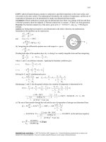
2-14E The power consumed by the resistance wire of an iron is given. The heat generation and the heat
flux are to be determined.
Assumptions Heat is generated uniformly in the resistance wire.

q = 1000 W
Analysis A 1000 W iron will convert electrical energy into

heat in the wire at a rate of 1000 W. Therefore, the rate of heat
D = 0.08 in
generation in a resistance wire is simply equal to the power
rating of a resistance heater. Then the rate of heat generation in
L = 15 in
the wire per unit volume is determined by dividing the total
rate of heat generation by the volume of the wire to be
E& gen
E& gen
1000 W
⎛ 3.412 Btu/h ⎞
7
3
=
=
e& gen =
⎜
⎟ = 7.820 × 10 Btu/h ⋅ ft
2
2
1W
V wire (πD / 4) L [π (0.08 / 12 ft) / 4](15 / 12 ft) ⎝
⎠
Similarly, heat flux on the outer surface of the wire as a result of this heat generation is determined by
dividing the total rate of heat generation by the surface area of the wire to be
E& gen
E& gen
1000 W
⎛ 3.412 Btu/h ⎞
5

2
=
=
q& =
⎜
⎟ = 1.303 × 10 Btu/h ⋅ ft
1W
Awire πDL π (0.08 / 12 ft)(15 / 12 ft) ⎝
⎠
Discussion Note that heat generation is expressed per unit volume in Btu/h⋅ft3 whereas heat flux is
expressed per unit surface area in Btu/h⋅ft2.

PROPRIETARY MATERIAL. © 2007 The McGraw-Hill Companies, Inc. Limited distribution permitted only to teachers and
educators for course preparation. If you are a student using this Manual, you are using it without permission.


2-4

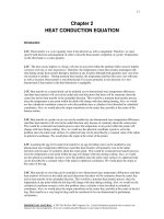
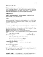
2-15E EES Prob. 2-14E is reconsidered. The surface heat flux as a function of wire diameter is to be
plotted.
Analysis The problem is solved using EES, and the solution is given below.
"GIVEN"
E_dot=1000 [W]
L=15 [in]
D=0.08 [in]
"ANALYSIS"
g_dot=E_dot/V_wire*Convert(W, Btu/h)
V_wire=pi*D^2/4*L*Convert(in^3, ft^3)
q_dot=E_dot/A_wire*Convert(W, Btu/h)
A_wire=pi*D*L*Convert(in^2, ft^2)

550000
500000
450000
400000
350000
2

0.02
0.04
0.06
0.08
0.1
0.12
0.14
0.16
0.18
0.2

q
[Btu/h.ft2]
521370
260685
173790
130342
104274
86895
74481
65171
57930
52137

q [Btu/h-ft ]

D [in]

300000
250000
200000
150000
100000
50000
0
0.02

0.04 0.06

0.08

0.1

0.12

0.14

0.16 0.18

0.2

D [in]

2-16 A certain thermopile used for heat flux meters is considered. The minimum heat flux this meter can
detect is to be determined.
Assumptions 1 Steady operating conditions exist.
Properties The thermal conductivity of kapton is given to be 0.345 W/m⋅K.
Analysis The minimum heat flux can be determined from
q& = k

Δt
0.1°C
= (0.345 W/m ⋅ °C)
= 17.3 W/m 2
L
0.002 m

PROPRIETARY MATERIAL. © 2007 The McGraw-Hill Companies, Inc. Limited distribution permitted only to teachers and
educators for course preparation. If you are a student using this Manual, you are using it without permission.


2-5

2-17 The rate of heat generation per unit volume in the uranium rods is given. The total rate of heat
generation in each rod is to be determined.
g = 7×107 W/m3
Assumptions Heat is generated uniformly in the uranium rods.
Analysis The total rate of heat generation in the rod is
determined by multiplying the rate of heat generation per unit
volume by the volume of the rod

D = 5 cm
L=1m

E& gen = e& genV rod = e& gen (πD 2 / 4) L = (7 × 10 7 W/m 3 )[π (0.05 m) 2 / 4](1 m) = 1.374 × 10 5 W = 137 kW

2-18 The variation of the absorption of solar energy in a solar pond with depth is given. A relation for the
total rate of heat generation in a water layer at the top of the pond is to be determined.
Assumptions Absorption of solar radiation by water is modeled as heat generation.
Analysis The total rate of heat generation in a water layer of surface area A and thickness L at the top of the
pond is determined by integration to be

E& gen =

∫V

e& gen dV =

∫

L

x =0

e& 0 e −bx ( Adx) = Ae&0

e −bx
−b

L

=
0

Ae& 0 (1 − e −bL )
b

2-19 The rate of heat generation per unit volume in a stainless steel plate is given. The heat flux on the
surface of the plate is to be determined.
Assumptions Heat is generated uniformly in steel plate.
Analysis We consider a unit surface area of 1 m2. The total rate of heat
generation in this section of the plate is
E& gen = e& genV plate = e& gen ( A × L ) = (5 × 10 6 W/m 3 )(1 m 2 )(0.03 m) = 1.5 × 10 5 W

e
L

Noting that this heat will be dissipated from both sides of the plate,
the heat flux on either surface of the plate becomes
E& gen 1.5 × 10 5 W
q& =
=
= 75,000 W/m 2 = 75 kW/m 2
2
Aplate
2 ×1 m

PROPRIETARY MATERIAL. © 2007 The McGraw-Hill Companies, Inc. Limited distribution permitted only to teachers and
educators for course preparation. If you are a student using this Manual, you are using it without permission.


2-6

Heat Conduction Equation

2-20 The one-dimensional transient heat conduction equation for a plane wall with constant thermal
∂ 2 T e& gen 1 ∂T
. Here T is the temperature, x is the space variable,
conductivity and heat generation is
+
=
k
α ∂t
∂x 2
e&gen is the heat generation per unit volume, k is the thermal conductivity, α is the thermal diffusivity, and t
is the time.
2-21 The one-dimensional transient heat conduction equation for a plane wall with constant thermal
1 ∂ ⎛ ∂T ⎞ e&gen 1 ∂T
conductivity and heat generation is
. Here T is the temperature, r is the space
=
⎜r
⎟+
k
r ∂r ⎝ ∂r ⎠
α ∂t
variable, g is the heat generation per unit volume, k is the thermal conductivity, α is the thermal diffusivity,
and t is the time.

2-22 We consider a thin element of thickness Δx in a large plane wall (see Fig. 2-13 in the text). The
density of the wall is ρ, the specific heat is c, and the area of the wall normal to the direction of heat
transfer is A. In the absence of any heat generation, an energy balance on this thin element of thickness Δx
during a small time interval Δt can be expressed as

ΔE element
Q& x − Q& x + Δx =
Δt

where
ΔE element = E t + Δt − E t = mc(Tt + Δt − Tt ) = ρcAΔx(Tt + Δt − Tt )

Substituting,
T
− Tt
Q& x − Q& x + Δx = ρcAΔx t + Δt
Δt

Dividing by AΔx gives
−

T
− Tt
1 Q& x + Δx − Q& x
= ρc t + Δt
A
Δx
Δt

Taking the limit as Δx → 0 and Δt → 0 yields
1 ∂ ⎛ ∂T ⎞
∂T
⎜ kA
⎟ = ρc
A ∂x ⎝

∂t
∂x ⎠

since from the definition of the derivative and Fourier’s law of heat conduction,

Q& x + Δx − Q& x ∂Q ∂ ⎛
∂T ⎞
=
=
⎜ − kA
⎟
Δx →0
Δx
∂x ∂x ⎝
∂x ⎠
lim

Noting that the area A of a plane wall is constant, the one-dimensional transient heat conduction equation
in a plane wall with constant thermal conductivity k becomes
∂ 2T
∂x

2

=

1 ∂T
α ∂t

where the property α = k / ρc is the thermal diffusivity of the material.

PROPRIETARY MATERIAL. © 2007 The McGraw-Hill Companies, Inc. Limited distribution permitted only to teachers and
educators for course preparation. If you are a student using this Manual, you are using it without permission.


2-7
2-23 We consider a thin cylindrical shell element of thickness Δr in a long cylinder (see Fig. 2-15 in the
text). The density of the cylinder is ρ, the specific heat is c, and the length is L. The area of the cylinder
normal to the direction of heat transfer at any location is A = 2πrL where r is the value of the radius at that
location. Note that the heat transfer area A depends on r in this case, and thus it varies with location. An
energy balance on this thin cylindrical shell element of thickness Δr during a small time interval Δt can be
expressed as
ΔE element
Q& r − Q& r + Δr + E& element =
Δt

where
ΔE element = E t + Δt − E t = mc(Tt + Δt − Tt ) = ρcAΔr (Tt + Δt − Tt )
E& element = e& genV element = e& gen AΔr

Substituting,
T
− Tt
Q& r − Q& r + Δr + e& gen AΔr = ρcAΔr t + Δt
Δt

where A = 2πrL . Dividing the equation above by AΔr gives
−

T

− Tt
1 Q& r + Δr − Q& r
+ e& gen = ρc t + Δt
A
Δr
Δt

Taking the limit as Δr → 0 and Δt → 0 yields
∂T
1 ∂ ⎛ ∂T ⎞
⎜ kA
⎟ + e& gen = ρc
∂r ⎠
A ∂r ⎝
∂t

since, from the definition of the derivative and Fourier’s law of heat conduction,

Q& r + Δr − Q& r ∂Q ∂ ⎛
∂T ⎞
=
= ⎜ − kA
⎟
Δr →0
Δr
∂r ∂r ⎝
∂r ⎠
lim

Noting that the heat transfer area in this case is A = 2πrL and the thermal conductivity is constant, the onedimensional transient heat conduction equation in a cylinder becomes

1 ∂ ⎛ ∂T ⎞
1 ∂T
⎜r
⎟ + e& gen =
r ∂r ⎝ ∂r ⎠
α ∂t

where α = k / ρc is the thermal diffusivity of the material.

PROPRIETARY MATERIAL. © 2007 The McGraw-Hill Companies, Inc. Limited distribution permitted only to teachers and
educators for course preparation. If you are a student using this Manual, you are using it without permission.


2-8
2-24 We consider a thin spherical shell element of thickness Δr in a sphere (see Fig. 2-17 in the text).. The
density of the sphere is ρ, the specific heat is c, and the length is L. The area of the sphere normal to the
direction of heat transfer at any location is A = 4πr 2 where r is the value of the radius at that location.
Note that the heat transfer area A depends on r in this case, and thus it varies with location. When there is
no heat generation, an energy balance on this thin spherical shell element of thickness Δr during a small
time interval Δt can be expressed as
ΔE element
Q& r − Q& r + Δr =
Δt

where
ΔE element = E t + Δt − E t = mc(Tt + Δt − Tt ) = ρcAΔr (Tt + Δt − Tt )

Substituting,
T
−T

Q& r − Q& r + Δr = ρcAΔr t + Δt t
Δt

where A = 4πr 2 . Dividing the equation above by AΔr gives
−

T
− Tt
1 Q& r + Δr − Q& r
= ρc t + Δt
A
Δr
Δt

Taking the limit as Δr → 0 and Δt → 0 yields
1 ∂ ⎛ ∂T ⎞
∂T
⎜ kA
⎟ = ρc
∂r ⎠
A ∂r ⎝
∂t

since, from the definition of the derivative and Fourier’s law of heat conduction,

Q& r + Δr − Q& r ∂Q ∂ ⎛
∂T ⎞
=
= ⎜ − kA
⎟

Δr →0
Δr
∂r ∂r ⎝
∂r ⎠
lim

Noting that the heat transfer area in this case is A = 4πr 2 and the thermal conductivity k is constant, the
one-dimensional transient heat conduction equation in a sphere becomes
1 ∂ ⎛ 2 ∂T ⎞ 1 ∂T
⎜r
⎟=
∂r ⎠ α ∂t
r 2 ∂r ⎝

where α = k / ρc is the thermal diffusivity of the material.

2-25 For a medium in which the heat conduction equation is given in its simplest by

∂ 2T
∂x

2

=

1 ∂T
:
α ∂t

(a) Heat transfer is transient, (b) it is one-dimensional, (c) there is no heat generation, and (d) the thermal

conductivity is constant.

PROPRIETARY MATERIAL. © 2007 The McGraw-Hill Companies, Inc. Limited distribution permitted only to teachers and
educators for course preparation. If you are a student using this Manual, you are using it without permission.


2-9

2-26 For a medium in which the heat conduction equation is given in its simplest by
1 d ⎛ dT ⎞
⎜ rk
⎟ + e& gen = 0 :
r dr ⎝ dr ⎠
(a) Heat transfer is steady, (b) it is one-dimensional, (c) there is heat generation, and (d) the thermal
conductivity is variable.

2-27 For a medium in which the heat conduction equation is given by

1 ∂ ⎛ 2 ∂T ⎞ 1 ∂T
⎜r
⎟=
∂r ⎠ α ∂t
r 2 ∂r ⎝

(a) Heat transfer is transient, (b) it is one-dimensional, (c) there is no heat generation, and (d) the thermal
conductivity is constant.

2-28 For a medium in which the heat conduction equation is given in its simplest by r

d 2T dT

+
=0:
dr 2 dr

(a) Heat transfer is steady, (b) it is one-dimensional, (c) there is no heat generation, and (d) the thermal
conductivity is constant.

PROPRIETARY MATERIAL. © 2007 The McGraw-Hill Companies, Inc. Limited distribution permitted only to teachers and
educators for course preparation. If you are a student using this Manual, you are using it without permission.


2-10
2-29 We consider a small rectangular element of length Δx, width Δy, and height Δz = 1 (similar to the one
in Fig. 2-21). The density of the body is ρ and the specific heat is c. Noting that heat conduction is twodimensional and assuming no heat generation, an energy balance on this element during a small time
interval Δt can be expressed as
Rate of heat ⎞ ⎛ Rate of heat conduction ⎞ ⎛ Rate of change of
⎛
⎜
⎟ ⎜
⎟ ⎜
at the surfaces at
⎜ conduction at the ⎟ − ⎜
⎟ = ⎜ the energy content
⎜ surfaces at x and y ⎟ ⎜ x + Δx and y + Δy
⎟ ⎜ of the element
⎝
⎠ ⎝
⎠ ⎝
or

⎞
⎟
⎟
⎟
⎠

ΔE element
Q& x + Q& y − Q& x + Δx − Q& y + Δy =
Δt

Noting that the volume of the element is V element = ΔxΔyΔz = ΔxΔy × 1 , the change in the energy content of
the element can be expressed as
ΔE element = E t + Δt − E t = mc(Tt + Δt − Tt ) = ρcΔxΔy (Tt + Δt − Tt )
T
− Tt
Q& x + Q& y − Q& x + Δx − Q& y + Δy = ρcΔxΔy t + Δt
Δt

Substituting,

Dividing by ΔxΔy gives
−

&
&
T
− Tt
1 Q& x + Δx − Q& x
1 Q y + Δy − Q y
−

= ρc t + Δt
Δy
Δx
Δx
Δy
Δt

Taking the thermal conductivity k to be constant and noting that the heat transfer surface areas of the
element for heat conduction in the x and y directions are Ax = Δy × 1 and A y = Δx × 1, respectively, and
taking the limit as Δx, Δy, and Δt → 0 yields
∂ 2T
∂x

2

+

∂ 2T
∂y

2

=

1 ∂T
α ∂t

since, from the definition of the derivative and Fourier’s law of heat conduction,

∂T ⎞

∂ ⎛ ∂T ⎞
1 Q& x + Δx − Q& x
1 ∂Q x
1 ∂ ⎛
∂ 2T
=
=
⎜ − kΔyΔz
⎟ = − ⎜k
⎟ = −k 2
Δx →0 ΔyΔz
Δx
ΔyΔz ∂x
ΔyΔz ∂x ⎝
∂x ⎠
∂x ⎝ ∂x ⎠
∂x
lim

&
&
1 Q y + Δy − Q y
1 ∂Q y
1 ∂ ⎛
∂ 2T
∂ ⎛ ∂T ⎞
∂T ⎞
⎟⎟ = − k
⎟⎟ = − ⎜⎜ k
⎜⎜ − kΔxΔz

=
=
Δy → 0 ΔxΔz
∂y ⎝ ∂y ⎠
Δy
ΔxΔz ∂y
ΔxΔz ∂y ⎝
∂y ⎠
∂y 2
lim

Here the property α = k / ρ c is the thermal diffusivity of the material.

PROPRIETARY MATERIAL. © 2007 The McGraw-Hill Companies, Inc. Limited distribution permitted only to teachers and
educators for course preparation. If you are a student using this Manual, you are using it without permission.


2-11

2-30 We consider a thin ring shaped volume element of width Δz and thickness Δr in a cylinder. The
density of the cylinder is ρ and the specific heat is c. In general, an energy balance on this ring element
during a small time interval Δt can be expressed as
ΔE element
(Q& r − Q& r + Δr ) + (Q& z − Q& z + Δz ) =
Δt

Δz

But the change in the energy content of the element can be expressed as
ΔE element = E t + Δt − E t = mc(Tt + Δt − Tt ) = ρc(2πrΔr )Δz (Tt + Δt − Tt )

rr

r+Δr

Substituting,
(Q& r − Q& r + Δr ) + (Q& z − Q& z + Δz ) = ρc ( 2πrΔr ) Δz

T t + Δt − Tt
Δt

Dividing the equation above by (2πrΔr )Δz gives
−

T
− Tt
1 Q& r + Δr − Q& r
1 Q& z + Δz − Q& z
−
= ρc t + Δt
2πrΔz
2πrΔr
Δr
Δz
Δt

Noting that the heat transfer surface areas of the element for heat conduction in the r and z directions are
Ar = 2πrΔz and Az = 2πrΔr , respectively, and taking the limit as Δr , Δz and Δt → 0 yields
∂T
1 ∂ ⎛ ∂T ⎞ 1 ∂ ⎛ ∂T ⎞ ∂ ⎛ ∂T ⎞

⎜⎜ k
⎟⎟ + ⎜ k
⎜ kr
⎟+ 2
⎟ = ρc
r ∂r ⎝ ∂r ⎠ r ∂φ ⎝ ∂φ ⎠ ∂z ⎝ ∂z ⎠
∂t

since, from the definition of the derivative and Fourier’s law of heat conduction,

∂ ⎛
∂T ⎞
1 Q& r + Δr − Q& r
1 ∂Q
1
1 ∂ ⎛ ∂T ⎞
=
=
⎜ − k (2πrΔz )
⎟=−
⎜ kr
⎟
Δr →0 2πrΔz
Δr
∂r ⎠
2πrΔz ∂r 2πrΔz ∂r ⎝
r ∂r ⎝ ∂r ⎠
lim

∂ ⎛

∂T ⎞
∂ ⎛ ∂T ⎞
1 Q& z + Δz − Q& z
1 ∂Qz
1
=
=
⎜ − k (2πrΔr )
⎟ = − ⎜k
⎟
Δz → 0 2πrΔr
Δz
∂z ⎠
∂z ⎝ ∂z ⎠
2πrΔr ∂z
2πrΔr ∂z ⎝
lim

For the case of constant thermal conductivity the equation above reduces to

1 ∂ ⎛ ∂T ⎞ ∂ 2 T 1 ∂T
=
⎜r
⎟+
r ∂r ⎝ ∂r ⎠ ∂z 2 α ∂t
where α = k / ρ c is the thermal diffusivity of the material. For the case of steady heat conduction with no
heat generation it reduces to

1 ∂ ⎛ ∂T ⎞ ∂ 2 T
=0

⎜r
⎟+
r ∂r ⎝ ∂r ⎠ ∂z 2

PROPRIETARY MATERIAL. © 2007 The McGraw-Hill Companies, Inc. Limited distribution permitted only to teachers and
educators for course preparation. If you are a student using this Manual, you are using it without permission.


2-12

2-31 Consider a thin disk element of thickness Δz and diameter D in a long cylinder (Fig. P2-31). The
density of the cylinder is ρ, the specific heat is c, and the area of the cylinder normal to the direction of heat
transfer is A = πD 2 / 4 , which is constant. An energy balance on this thin element of thickness Δz during a
small time interval Δt can be expressed as
⎛ Rate of heat ⎞ ⎛ Rate of heat
⎜
⎟ ⎜
⎜ conduction at ⎟ − ⎜ conduction at the
⎜ the surface at z ⎟ ⎜ surface at z + Δz
⎝
⎠ ⎝

⎞ ⎛ Rate of heat ⎞ ⎛ Rate of change of
⎟ ⎜
⎟ ⎜
⎟ + ⎜ generation inside ⎟ = ⎜ the energy content
⎟ ⎜ the element ⎟ ⎜ of the element
⎠ ⎝
⎠ ⎝

⎞
⎟
⎟
⎟
⎠

or,
ΔE element
Q& z − Q& z + Δz + E& element =
Δt

But the change in the energy content of the element and the rate of heat generation within the element can
be expressed as
ΔE element = E t + Δt − E t = mc(Tt + Δt − Tt ) = ρcAΔz (Tt + Δt − Tt )

and
E& element = e& genV element = e& gen AΔz

Substituting,
T
− Tt
Q& z − Q& z + Δz + e& gen AΔz = ρcAΔz t + Δt
Δt

Dividing by AΔz gives
−

T
− Tt
1 Q& z + Δz − Q& z

+ e& gen = ρc t + Δt
A
Δz
Δt

Taking the limit as Δz → 0 and Δt → 0 yields
∂T
1 ∂ ⎛ ∂T ⎞
⎜ kA
⎟ + e& gen = ρc
∂z ⎠
A ∂z ⎝
∂t

since, from the definition of the derivative and Fourier’s law of heat conduction,
Q& z + Δz − Q& z ∂Q ∂ ⎛
∂T ⎞
=
=
⎜ − kA
⎟
Δz → 0
Δz
∂z ∂z ⎝
∂z ⎠
lim

Noting that the area A and the thermal conductivity k are constant, the one-dimensional transient heat
conduction equation in the axial direction in a long cylinder becomes
∂ 2T

∂z

2

+

e& gen
k

=

1 ∂T
α ∂t

where the property α = k / ρc is the thermal diffusivity of the material.

PROPRIETARY MATERIAL. © 2007 The McGraw-Hill Companies, Inc. Limited distribution permitted only to teachers and
educators for course preparation. If you are a student using this Manual, you are using it without permission.


2-13

2-32 For a medium in which the heat conduction equation is given by

∂ 2T
∂x

2

+

∂ 2T
∂y

2

=

1 ∂T
:
α ∂t

(a) Heat transfer is transient, (b) it is two-dimensional, (c) there is no heat generation, and (d) the thermal
conductivity is constant.

2-33
1 ∂
r ∂r

For a medium in which the heat conduction equation is given by
⎛ ∂T ⎞ ∂ ⎛ ∂T ⎞
⎜ kr
⎟ + ⎜k
⎟ + e& gen = 0 :
⎝ ∂r ⎠ ∂z ⎝ ∂z ⎠

(a) Heat transfer is steady, (b) it is two-dimensional, (c) there is heat generation, and (d) the thermal
conductivity is variable.

2-34 For a medium in which the heat conduction equation is given by

1 ∂ ⎛ 2 ∂T ⎞
1
∂ 2 T 1 ∂T
=
⎜r
⎟+ 2
2 ∂r
2
∂r ⎠ r sin θ ∂φ 2 α ∂t
r
⎝
(a) Heat transfer is transient, (b) it is two-dimensional, (c) there is no heat generation, and (d) the thermal
conductivity is constant.

Boundary and Initial Conditions; Formulation of Heat Conduction Problems

2-35C The mathematical expressions of the thermal conditions at the boundaries are called the boundary
conditions. To describe a heat transfer problem completely, two boundary conditions must be given for
each direction of the coordinate system along which heat transfer is significant. Therefore, we need to
specify four boundary conditions for two-dimensional problems.
2-36C The mathematical expression for the temperature distribution of the medium initially is called the
initial condition. We need only one initial condition for a heat conduction problem regardless of the
dimension since the conduction equation is first order in time (it involves the first derivative of temperature
with respect to time). Therefore, we need only 1 initial condition for a two-dimensional problem.
2-37C A heat transfer problem that is symmetric about a plane, line, or point is said to have thermal
symmetry about that plane, line, or point. The thermal symmetry boundary condition is a mathematical
expression of this thermal symmetry. It is equivalent to insulation or zero heat flux boundary condition, and
is expressed at a point x0 as ∂T ( x 0 , t ) / ∂x = 0 .

PROPRIETARY MATERIAL. © 2007 The McGraw-Hill Companies, Inc. Limited distribution permitted only to teachers and

educators for course preparation. If you are a student using this Manual, you are using it without permission.


2-14

2-38C The boundary condition at a perfectly insulated surface (at x = 0, for example) can be expressed as
−k

∂ T ( 0, t )
=0
∂x

or

∂ T ( 0, t )
= 0 which indicates zero heat flux.
∂x

2-39C Yes, the temperature profile in a medium must be perpendicular to an insulated surface since the
slope ∂T / ∂x = 0 at that surface.
2-40C We try to avoid the radiation boundary condition in heat transfer analysis because it is a non-linear
expression that causes mathematical difficulties while solving the problem; often making it impossible to
obtain analytical solutions.

2-41 A spherical container of inner radius r1 , outer radius r2 , and thermal
conductivity k is given. The boundary condition on the inner surface of the
container for steady one-dimensional conduction is to be expressed for the
following cases:

r1

r2

(a) Specified temperature of 50°C: T ( r1 ) = 50°C
(b) Specified heat flux of 30 W/m2 towards the center: k

dT ( r1 )
= 30 W/m 2
dr

(c) Convection to a medium at T∞ with a heat transfer coefficient of h: k

dT (r1 )
= h[T (r1 ) − T∞ ]
dr

2-42 Heat is generated in a long wire of radius ro covered with a plastic insulation layer at a constant rate
of e&gen . The heat flux boundary condition at the interface (radius ro) in terms of the heat generated is to be
expressed. The total heat generated in the wire and the heat flux at the interface are
E& gen = e& genV wire = e& gen (πro2 L)
q& s =

2
Q& s E& gen e& gen (πro L) e& gen ro
=
=
=
A
A
(2πro ) L

2

D

egen

L

Assuming steady one-dimensional conduction in the radial direction, the heat flux boundary condition can
be expressed as
−k

dT (ro ) e&gen ro
=
dr
2

PROPRIETARY MATERIAL. © 2007 The McGraw-Hill Companies, Inc. Limited distribution permitted only to teachers and
educators for course preparation. If you are a student using this Manual, you are using it without permission.


2-15

2-43 A long pipe of inner radius r1, outer radius r2, and thermal conductivity
k is considered. The outer surface of the pipe is subjected to convection to a
medium at T∞ with a heat transfer coefficient of h. Assuming steady onedimensional conduction in the radial direction, the convection boundary
condition on the outer surface of the pipe can be expressed as
−k

r1

r2

dT ( r2 )
= h[T ( r2 ) − T∞ ]
dr

2-44 A spherical shell of inner radius r1, outer radius r2, and thermal
conductivity k is considered. The outer surface of the shell is
subjected to radiation to surrounding surfaces at Tsurr . Assuming no
convection and steady one-dimensional conduction in the radial
direction, the radiation boundary condition on the outer surface of the
shell can be expressed as
−k

h, T∞

[

dT ( r2 )
4
= εσ T ( r2 ) 4 − Tsurr
dr

ε
k
r1

Tsurr

r2

]

2-45 A spherical container consists of two spherical layers A and B that
are at perfect contact. The radius of the interface is ro. Assuming transient
one-dimensional conduction in the radial direction, the boundary
conditions at the interface can be expressed as

ro

T A ( ro , t ) = T B (ro , t )

and

−kA

∂T A (ro , t )
∂T B (ro , t )
= −k B
∂r
∂r

PROPRIETARY MATERIAL. © 2007 The McGraw-Hill Companies, Inc. Limited distribution permitted only to teachers and
educators for course preparation. If you are a student using this Manual, you are using it without permission.


2-16

2-46 Heat conduction through the bottom section of a steel pan that is used to boil water on top of an

electric range is considered. Assuming constant thermal conductivity and one-dimensional heat transfer,
the mathematical formulation (the differential equation and the boundary conditions) of this heat
conduction problem is to be obtained for steady operation.
Assumptions 1 Heat transfer is given to be steady and one-dimensional. 2 Thermal conductivity is given to
be constant. 3 There is no heat generation in the medium. 4 The top surface at x = L is subjected to
convection and the bottom surface at x = 0 is subjected to uniform heat flux.
Analysis The heat flux at the bottom of the pan is
E& gen
Q&
0.85 × (1250 W)
q& s = s =
=
= 33,820 W/m 2
2
As πD / 4 π (0.20 m) 2 / 4

Then the differential equation and the boundary conditions for this heat conduction problem can be
expressed as
d 2T
=0
dx 2

dT (0)
= q& s = 33,280 W/m 2
dx
dT ( L)
−k
= h[T ( L) − T∞ ]
dx
−k

2-47E A 2-kW resistance heater wire is used for space heating. Assuming constant thermal conductivity
and one-dimensional heat transfer, the mathematical formulation (the differential equation and the
boundary conditions) of this heat conduction problem is to be obtained for steady operation.
Assumptions 1 Heat transfer is given to be steady and one-dimensional. 2 Thermal conductivity is given to
be constant. 3 Heat is generated uniformly in the wire.
Analysis The heat flux at the surface of the wire is
E& gen
Q&
1200 W
=
= 212.2 W/in 2
q& s = s =
As 2πro L 2π (0.06 in)(15 in)

Noting that there is thermal symmetry about the center line and there is uniform heat flux at the outer
surface, the differential equation and the boundary conditions for this heat conduction problem can be
expressed as
1 d ⎛ dT ⎞ e& gen
=0
⎜r
⎟+
r dr ⎝ dr ⎠
k

dT (0)
=0
dr
dT (ro )
−k

= q& s = 212.2 W/in 2
dr

2 kW
D = 0.12 in
L = 15 in

PROPRIETARY MATERIAL. © 2007 The McGraw-Hill Companies, Inc. Limited distribution permitted only to teachers and
educators for course preparation. If you are a student using this Manual, you are using it without permission.


2-17

2-48 Heat conduction through the bottom section of an aluminum pan that is used to cook stew on top of an
electric range is considered (Fig. P2-48). Assuming variable thermal conductivity and one-dimensional
heat transfer, the mathematical formulation (the differential equation and the boundary conditions) of this
heat conduction problem is to be obtained for steady operation.
Assumptions 1 Heat transfer is given to be steady and one-dimensional. 2 Thermal conductivity is given to
be variable. 3 There is no heat generation in the medium. 4 The top surface at x = L is subjected to
specified temperature and the bottom surface at x = 0 is subjected to uniform heat flux.
Analysis The heat flux at the bottom of the pan is
E& gen
Q&
0.90 × (900 W)
q& s = s =
=
= 31,831 W/m 2
2
As πD / 4 π (0.18 m) 2 / 4

Then the differential equation and the boundary conditions for this heat conduction problem can be
expressed as
d ⎛ dT ⎞
⎜k
⎟=0
dx ⎝ dx ⎠

−k

dT (0)
= q& s = 31,831 W/m 2
dx
T ( L) = TL = 108°C

2-49 Water flows through a pipe whose outer surface is wrapped with a thin electric heater that consumes
300 W per m length of the pipe. The exposed surface of the heater is heavily insulated so that the entire
heat generated in the heater is transferred to the pipe. Heat is transferred from the inner surface of the pipe
to the water by convection. Assuming constant thermal conductivity and one-dimensional heat transfer, the
mathematical formulation (the differential equation and the boundary conditions) of the heat conduction in
the pipe is to be obtained for steady operation.
Assumptions 1 Heat transfer is given to be steady and one-dimensional. 2 Thermal conductivity is given to
be constant. 3 There is no heat generation in the medium. 4 The outer surface at r = r2 is subjected to
uniform heat flux and the inner surface at r = r1 is subjected to convection.
Analysis The heat flux at the outer surface of the pipe is
q& s =

Q& s
Q& s
300 W
=

=
= 734.6 W/m 2
As 2πr2 L 2π (0.065 cm)(1 m)

Noting that there is thermal symmetry about the center line and
there is uniform heat flux at the outer surface, the differential
equation and the boundary conditions for this heat conduction
problem can be expressed as
d ⎛ dT ⎞
⎜r
⎟=0
dr ⎝ dr ⎠

Q = 300 W
h
T∞

r1

r2

dT ( r1 )
= h[T (ri ) − T∞ ] = 85[T (ri ) − 70]
dr
dT (r2 )
k
= q& s = 734.6 W/m 2
dr
k

PROPRIETARY MATERIAL. © 2007 The McGraw-Hill Companies, Inc. Limited distribution permitted only to teachers and
educators for course preparation. If you are a student using this Manual, you are using it without permission.


2-18

2-50 A spherical metal ball that is heated in an oven to a temperature of Ti throughout is dropped into a
large body of water at T∞ where it is cooled by convection. Assuming constant thermal conductivity and
transient one-dimensional heat transfer, the mathematical formulation (the differential equation and the
boundary and initial conditions) of this heat conduction problem is to be obtained.
Assumptions 1 Heat transfer is given to be transient and one-dimensional. 2 Thermal conductivity is given
to be constant. 3 There is no heat generation in the medium. 4 The outer surface at r = r0 is subjected to
convection.
Analysis Noting that there is thermal symmetry about the midpoint and convection at the outer surface,
the differential equation and the boundary conditions for this heat conduction problem can be expressed as
1 ∂ ⎛ 2 ∂T ⎞ 1 ∂T
⎜r
⎟=
∂r ⎠ α ∂t
r 2 ∂r ⎝

∂T (0, t )
=0
∂r
∂T (ro , t )
−k
= h[T (ro ) − T∞ ]
∂r
T (r ,0) = Ti

k

T∞
h

r2

Ti

2-51 A spherical metal ball that is heated in an oven to a temperature of Ti throughout is allowed to cool
in ambient air at T∞ by convection and radiation. Assuming constant thermal conductivity and transient
one-dimensional heat transfer, the mathematical formulation (the differential equation and the boundary
and initial conditions) of this heat conduction problem is to be obtained.
Assumptions 1 Heat transfer is given to be transient and one-dimensional. 2 Thermal conductivity is given
to be variable. 3 There is no heat generation in the medium. 4 The outer surface at r = ro is subjected to
convection and radiation.
Analysis Noting that there is thermal symmetry about the midpoint and convection and radiation at the
outer surface and expressing all temperatures in Rankine, the differential equation and the boundary
conditions for this heat conduction problem can be expressed as

ε

1 ∂ ⎛ 2 ∂T ⎞
∂T
⎜ kr
⎟ = ρc
2 ∂r
∂r ⎠
∂t
r

⎝

∂T (0, t )
=0
∂r
∂T (ro , t )
4
−k
= h[T ( ro ) − T∞ ] + εσ[T (ro ) 4 − Tsurr
]
∂r
T (r ,0) = Ti

Tsurr
k

r2

T∞
h

Ti

PROPRIETARY MATERIAL. © 2007 The McGraw-Hill Companies, Inc. Limited distribution permitted only to teachers and
educators for course preparation. If you are a student using this Manual, you are using it without permission.


2-19

2-52 The outer surface of the East wall of a house exchanges heat with both convection and radiation.,

while the interior surface is subjected to convection only. Assuming the heat transfer through the wall to
be steady and one-dimensional, the mathematical formulation (the differential equation and the boundary
and initial conditions) of this heat conduction problem is to be obtained.
Assumptions 1 Heat transfer is given to be steady and onedimensional. 2 Thermal conductivity is given to be constant. 3
There is no heat generation in the medium. 4 The outer surface at x
= L is subjected to convection and radiation while the inner
surface at x = 0 is subjected to convection only.
Analysis Expressing all the temperatures in Kelvin, the differential
equation and the boundary conditions for this heat conduction
problem can be expressed as
d 2T
dx 2

Tsky
T∞1
h1

T∞2
h2

=0

−k

dT (0)
= h1[T∞1 − T (0)]
dx

−k

dT ( L)
4
= h1 [T ( L) − T∞ 2 ] + ε 2σ T ( L) 4 − Tsky
dx

L

[

x

]

Solution of Steady One-Dimensional Heat Conduction Problems

2-53C Yes, this claim is reasonable since in the absence of any heat generation the rate of heat transfer
through a plain wall in steady operation must be constant. But the value of this constant must be zero since
one side of the wall is perfectly insulated. Therefore, there can be no temperature difference between
different parts of the wall; that is, the temperature in a plane wall must be uniform in steady operation.
2-54C Yes, the temperature in a plane wall with constant thermal conductivity and no heat generation will
vary linearly during steady one-dimensional heat conduction even when the wall loses heat by radiation
from its surfaces. This is because the steady heat conduction equation in a plane wall is d 2T / dx 2 = 0
whose solution is T ( x ) = C1 x + C 2 regardless of the boundary conditions. The solution function represents
a straight line whose slope is C1.
2-55C Yes, in the case of constant thermal conductivity and no heat generation, the temperature in a solid
cylindrical rod whose ends are maintained at constant but different temperatures while the side surface is
perfectly insulated will vary linearly during steady one-dimensional heat conduction. This is because the
steady heat conduction equation in this case is d 2T / dx 2 = 0 whose solution is T ( x ) = C1 x + C 2 which
represents a straight line whose slope is C1.
2-56C Yes, this claim is reasonable since no heat is entering the cylinder and thus there can be no heat

transfer from the cylinder in steady operation. This condition will be satisfied only when there are no
temperature differences within the cylinder and the outer surface temperature of the cylinder is the equal to
the temperature of the surrounding medium.

PROPRIETARY MATERIAL. © 2007 The McGraw-Hill Companies, Inc. Limited distribution permitted only to teachers and
educators for course preparation. If you are a student using this Manual, you are using it without permission.


2-20

2-57 A large plane wall is subjected to specified temperature on the left surface and convection on the right
surface. The mathematical formulation, the variation of temperature, and the rate of heat transfer are to be
determined for steady one-dimensional heat transfer.
Assumptions 1 Heat conduction is steady and one-dimensional. 2 Thermal conductivity is constant. 3
There is no heat generation.
Properties The thermal conductivity is given to be k = 2.3 W/m⋅°C.
Analysis (a) Taking the direction normal to the surface of the wall to be the x direction with x = 0 at the left
surface, the mathematical formulation of this problem can be expressed as
d 2T
dx 2

=0

k

and

T1=90°C
A=30 m2

T (0) = T1 = 90°C
−k

dT ( L)
= h[T ( L) − T∞ ]
dx

L=0.4 m

T∞ =25°C
h=24 W/m2.°C

(b) Integrating the differential equation twice with respect to x yields
dT
= C1
dx

x

T ( x) = C1x + C2

where C1 and C2 are arbitrary constants. Applying the boundary conditions give
x = 0:

T (0) = C1 × 0 + C 2 → C 2 = T1

x = L:

− kC1 = h[(C1 L + C 2 ) − T∞ ] → C1 = −

h(C 2 − T∞ )
h(T1 − T∞ )
→ C1 = −
k + hL
k + hL

Substituting C1 and C 2 into the general solution, the variation of temperature is determined to be
T ( x) = −
=−

h(T1 − T∞ )
x + T1
k + hL
(24 W/m 2 ⋅ °C)(90 − 25)°C

(2.3 W/m ⋅ °C) + (24 W/m 2 ⋅ °C)(0.4 m)
= 90 − 131.1x

x + 90°C

(c) The rate of heat conduction through the wall is
h(T1 − T∞ )
dT
= −kAC1 = kA
Q& wall = −kA
dx
k + hL
(24 W/m 2 ⋅ °C)(90 − 25)°C
= (2.3 W/m ⋅ °C)(30 m 2 )
(2.3 W/m ⋅ °C) + (24 W/m 2 ⋅ °C)(0.4 m)

= 9045 W

Note that under steady conditions the rate of heat conduction through a plain wall is constant.

PROPRIETARY MATERIAL. © 2007 The McGraw-Hill Companies, Inc. Limited distribution permitted only to teachers and
educators for course preparation. If you are a student using this Manual, you are using it without permission.


2-21

2-58 The top and bottom surfaces of a solid cylindrical rod are maintained at constant temperatures of 20°C
and 95°C while the side surface is perfectly insulated. The rate of heat transfer through the rod is to be
determined for the cases of copper, steel, and granite rod.
Assumptions 1 Heat conduction is steady and one-dimensional. 2 Thermal conductivity is constant. 3
There is no heat generation.
Properties The thermal conductivities are given to be k = 380 W/m⋅°C for copper, k = 18 W/m⋅°C for
steel, and k = 1.2 W/m⋅°C for granite.
Analysis Noting that the heat transfer area (the area normal to
the direction of heat transfer) is constant, the rate of heat
transfer along the rod is determined from
T − T2
Q& = kA 1
L

T1=25°C

Insulated

D = 0.05 m

T2=95°C

where L = 0.15 m and the heat transfer area A is
A = πD 2 / 4 = π (0.05 m) 2 / 4 = 1.964 × 10 −3 m 2

L=0.15 m

Then the heat transfer rate for each case is determined as follows:
(a) Copper:

T − T2
(95 − 20)°C
Q& = kA 1
= (380 W/m ⋅ °C)(1.964 × 10 −3 m 2 )
= 373.1 W
L
0.15 m

(b) Steel:

T − T2
(95 − 20)°C
Q& = kA 1
= (18 W/m ⋅ °C)(1.964 × 10 −3 m 2 )
= 17.7 W
L
0.15 m

(c) Granite:

T − T2
(95 − 20)°C
Q& = kA 1
= (1.2 W/m ⋅ °C)(1.964 × 10 −3 m 2 )
= 1.2 W
L
0.15 m

Discussion: The steady rate of heat conduction can differ by orders of magnitude, depending on the
thermal conductivity of the material.

PROPRIETARY MATERIAL. © 2007 The McGraw-Hill Companies, Inc. Limited distribution permitted only to teachers and
educators for course preparation. If you are a student using this Manual, you are using it without permission.


2-22

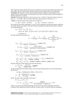
2-59 EES Prob. 2-58 is reconsidered. The rate of heat transfer as a function of the thermal conductivity of
the rod is to be plotted.
Analysis The problem is solved using EES, and the solution is given below.
"GIVEN"
L=0.15 [m]
D=0.05 [m]
T_1=20 [C]
T_2=95 [C]
k=1.2 [W/m-C]
"ANALYSIS"
A=pi*D^2/4
Q_dot=k*A*(T_2-T_1)/L

Q [W]
0.9817
21.6
42.22
62.83
83.45
104.1
124.7
145.3
165.9
186.5
207.1
227.8
248.4
269
289.6
310.2
330.8
351.5
372.1
392.7

400
350
300
250

Q [W ]

k [W/m.C]

1
22
43
64
85
106
127
148
169
190
211
232
253
274
295
316
337
358
379
400

200
150
100
50
0
0

50

100

150

200

250

300

350

400

k [W /m -C]

PROPRIETARY MATERIAL. © 2007 The McGraw-Hill Companies, Inc. Limited distribution permitted only to teachers and
educators for course preparation. If you are a student using this Manual, you are using it without permission.


2-23

2-60 The base plate of a household iron is subjected to specified heat flux on the left surface and to
specified temperature on the right surface. The mathematical formulation, the variation of temperature in
the plate, and the inner surface temperature are to be determined for steady one-dimensional heat transfer.
Assumptions 1 Heat conduction is steady and one-dimensional since the surface area of the base plate is
large relative to its thickness, and the thermal conditions on both sides of the plate are uniform. 2 Thermal
conductivity is constant. 3 There is no heat generation in the plate. 4 Heat loss through the upper part of
the iron is negligible.
Properties The thermal conductivity is given to be k = 20 W/m⋅°C.

Analysis (a) Noting that the upper part of the iron is well insulated and thus the entire heat generated in the
resistance wires is transferred to the base plate, the heat flux through the inner surface is determined to be

q& 0 =

Q& 0
800 W
=
= 50,000 W/m 2
Abase 160 ×10 − 4 m 2

Taking the direction normal to the surface of the wall to be the x direction with x = 0 at the left surface, the
mathematical formulation of this problem can be expressed as
d 2T
=0
dx 2

and

−k

dT (0)
= q& 0 = 50,000 W/m 2
dx

T ( L) = T2 = 85°C

(b) Integrating the differential equation twice with respect to x yields
dT
= C1

dx

T ( x) = C1x + C2

where C1 and C2 are arbitrary constants. Applying the boundary conditions give
q& 0
k

x = 0:

− kC1 = q& 0 → C1 = −

x = L:

T ( L) = C1 L + C 2 = T2 → C 2 = T2 − C1 L → C 2 = T2 +

q& 0 L
k

Substituting C1 and C 2 into the general solution, the variation of temperature is determined to be
T ( x) = −

q& 0
q& L q& ( L − x)
x + T2 + 0 = 0
+ T2
k
k
k

(50,000 W/m 2 )(0.006 − x)m
+ 85°C
20 W/m ⋅ °C
= 2500(0.006 − x) + 85

=

(c) The temperature at x = 0 (the inner surface of the plate) is
T (0) = 2500(0.006 − 0) + 85 = 100°C

Note that the inner surface temperature is higher than the exposed surface temperature, as expected.

PROPRIETARY MATERIAL. © 2007 The McGraw-Hill Companies, Inc. Limited distribution permitted only to teachers and
educators for course preparation. If you are a student using this Manual, you are using it without permission.


2-24

2-61 The base plate of a household iron is subjected to specified heat flux on the left surface and to
specified temperature on the right surface. The mathematical formulation, the variation of temperature in
the plate, and the inner surface temperature are to be determined for steady one-dimensional heat transfer.
Assumptions 1 Heat conduction is steady and one-dimensional since the surface area of the base plate is
large relative to its thickness, and the thermal conditions on both sides of the plate are uniform. 2 Thermal
conductivity is constant. 3 There is no heat generation in the plate. 4 Heat loss through the upper part of
the iron is negligible.
Properties The thermal conductivity is given to be k = 20 W/m⋅°C.
Analysis (a) Noting that the upper part of the iron is well
insulated and thus the entire heat generated in the resistance
wires is transferred to the base plate, the heat flux through
the inner surface is determined to be

q& 0 =

Q& 0
1200 W
=
= 75,000 W/m 2
Abase 160 ×10 − 4 m 2

Q=1200 W
A=160 cm2

k

T2 =85°C

L=0.6 cm

Taking the direction normal to the surface of the wall to be the
x direction with x = 0 at the left surface, the mathematical
formulation of this problem can be expressed as

x

d 2T
=0
dx 2

and

−k

dT (0)
= q& 0 = 75,000 W/m 2
dx

T ( L) = T2 = 85°C

(b) Integrating the differential equation twice with respect to x yields
dT
= C1
dx

T ( x) = C1x + C2

where C1 and C2 are arbitrary constants. Applying the boundary conditions give
q& 0
k

x = 0:

− kC1 = q& 0 → C1 = −

x = L:

T ( L) = C1 L + C 2 = T2 → C 2 = T2 − C1 L → C 2 = T2 +

q& 0 L
k

Substituting C1 and C2 into the general solution, the variation of temperature is determined to be
T ( x) = −

q& L q& ( L − x)
q& 0
x + T2 + 0 = 0
+ T2
k
k
k

(75,000 W/m 2 )(0.006 − x)m
+ 85°C
20 W/m ⋅ °C
= 3750(0.006 − x) + 85
=

(c) The temperature at x = 0 (the inner surface of the plate) is
T (0) = 3750(0.006 − 0) + 85 = 107.5°C

Note that the inner surface temperature is higher than the exposed surface temperature, as expected.

PROPRIETARY MATERIAL. © 2007 The McGraw-Hill Companies, Inc. Limited distribution permitted only to teachers and
educators for course preparation. If you are a student using this Manual, you are using it without permission.


2-25

2-62 EES Prob. 2-60 is reconsidered. The temperature as a function of the distance is to be plotted.
Analysis The problem is solved using EES, and the solution is given below.

"GIVEN"
Q_dot=800 [W]
L=0.006 [m]
A_base=160E-4 [m^2]
k=20 [W/m-C]
T_2=85 [C]
"ANALYSIS"
q_dot_0=Q_dot/A_base
T=q_dot_0*(L-x)/k+T_2 "Variation of temperature"
"x is the parameter to be varied"

x [m]
0
0.0006667
0.001333
0.002
0.002667
0.003333
0.004
0.004667
0.005333
0.006

T [C]
100
98.33
96.67
95
93.33
91.67

90
88.33
86.67
85

100
98
96

T [C]

94
92
90
88
86
84
0

0.001

0.002

0.003

0.004

0.005

0.006

x [m ]

PROPRIETARY MATERIAL. © 2007 The McGraw-Hill Companies, Inc. Limited distribution permitted only to teachers and
educators for course preparation. If you are a student using this Manual, you are using it without permission.