Solution manual heat and mass transfer a practical approach 3rd edition cengel CH05 2

5-68

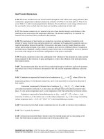
5-86 A uranium plate initially at a uniform temperature is subjected to insulation on one side and
convection on the other. The transient finite difference formulation of this problem is to be obtained, and
the nodal temperatures after 5 min and under steady conditions are to be determined.
Assumptions 1 Heat transfer is one-dimensional since the plate is large relative to its thickness. 2 Thermal
conductivity is constant. 3 Radiation heat transfer is negligible.
Properties The conductivity and diffusivity are given to be k = 28 W/m⋅°C and α = 12.5 × 10 −6 m 2 /s .
Analysis The nodal spacing is given to be Δx = 0.02 m. Then the number of nodes becomes M = L / Δx + 1
= 0.08/0.02+1 = 5. This problem involves 5 unknown nodal temperatures, and thus we need to have 5
equations. Node 0 is on insulated boundary, and thus we can treat it as an interior note by using the mirror
image concept. Nodes 1, 2, and 3 are interior nodes, and thus for them we can use the general explicit finite
difference relation expressed as
Tmi −1 − 2Tmi + Tmi +1 +

e& mi Δx 2 Tmi +1 − Tmi
=
k
τ

→ Tmi +1 = τ (Tmi −1 + Tmi +1 ) + (1 − 2τ )Tmi + τ

e& mi Δx 2
k

e

Insulated

The finite difference equation for node 4 on the right surface
subjected to convection is obtained by applying an energy

balance on the half volume element about node 4 and taking
the direction of all heat transfers to be towards the node under
consideration:

h, T∞

Δx
•
0

•
1

•
2

•
3

4

•

e& 0 Δx 2
k
&
e Δx 2
T1i +1 = τ (T0i + T2i ) + (1 − 2τ )T1i + τ 0
k
e& Δx 2

T2i +1 = τ (T1i + T3i ) + (1 − 2τ )T2i + τ 0
k
&
e Δx 2
T3i +1 = τ (T2i + T4i ) + (1 − 2τ )T3i + τ 0
k
i
i
T − T4
T i +1 − T4i
Δx
Δx
h(T∞ − T4i ) + k 3
+ e& 0
=ρ
cp 4
Δx
2
2
Δt

T0i +1 = τ (T1i + T1i ) + (1 − 2τ )T0i + τ

Node 0 (insulated) :
Node 1 (interior) :
Node 2 (interior) :
Node 3 (interior) :
Node 4 (convection) :

e& (Δx) 2

hΔx ⎞ i
hΔx
⎛
i
T4i +1 = ⎜1 − 2τ − 2τ
T∞ + τ 0
⎟T4 + 2τT3 + 2τ
k ⎠
k
k
⎝

or

where Δx = 0.02 m, e&0 = 10 6 W/m 3 , k = 28 W/m ⋅ °C, h = 35 W/m 2 ⋅ °C, T∞ = 20°C , and α = 12.5 × 10 −6
m2/s. The upper limit of the time step Δt is determined from the stability criteria that requires all primary
coefficients to be greater than or equal to zero. The coefficient of T4i is smaller in this case, and thus the
stability criteria for this problem can be expressed as

1 − 2τ − 2τ

hΔx
≥0 →
k

τ≤

1
2(1 + hΔx / k )

→ Δt ≤

Δx 2
2α (1 + hΔx / k )

since τ = αΔt / Δx 2 . Substituting the given quantities, the maximum allowable the time step becomes
Δt ≤

(0.02 m) 2
2(12.5 × 10 −6 m 2 /s)[1 + (35 W/m 2 .°C)(0.02 m) /( 28 W/m.°C)]

= 15.6 s

PROPRIETARY MATERIAL. © 2007 The McGraw-Hill Companies, Inc. Limited distribution permitted only to teachers and
educators for course preparation. If you are a student using this Manual, you are using it without permission.


5-69

Therefore, any time step less than 15.6 s can be used to solve this problem. For convenience, let us choose
the time step to be Δt = 15 s. Then the mesh Fourier number becomes

τ=

αΔt
Δx 2

=

(12.5 × 10 −6 m 2 /s)(15 s)

(0.02 m) 2

= 0.46875

Substituting this value of τ and other given quantities, the nodal temperatures after 5×60/15 = 20 time
steps (5 min) are determined to be
After 5 min: T0 = 228.9°C,

T1 = 228.4°C,

T2 = 226.8°C,

T3 = 224.0°C, and T4 = 219.9 °C

(b) The time needed for transient operation to be established is determined by increasing the number of
time steps until the nodal temperatures no longer change. In this case the nodal temperatures under steady
conditions are determined to be
T0 = 2420°C,

T1 = 2413°C,

T2 = 2391°C,

T3 = 2356°C,

and

T4 = 2306 °C

Discussion The steady solution can be checked independently by obtaining the steady finite difference

formulation, and solving the resulting equations simultaneously.

PROPRIETARY MATERIAL. © 2007 The McGraw-Hill Companies, Inc. Limited distribution permitted only to teachers and
educators for course preparation. If you are a student using this Manual, you are using it without permission.


5-70

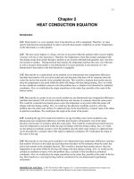
5-87 EES Prob. 5-86 is reconsidered. The effect of the cooling time on the temperatures of the left and
right sides of the plate is to be investigated.
Analysis The problem is solved using EES, and the solution is given below.
"GIVEN"
L=0.08 [m]
k=28 [W/m-C]
alpha=12.5E-6 [m^2/s]
T_i=100 [C]
g_dot=1E6 [W/m^3]
T_infinity=20 [C]
h=35 [W/m^2-C]
DELTAx=0.02 [m]
time=300 [s]
"ANALYSIS"
M=L/DELTAx+1 "Number of nodes"
DELTAt=15 "[s]"
tau=(alpha*DELTAt)/DELTAx^2
"The technique is to store the temperatures in the parametric table and recover them (as old
temperatures)
using the variable ROW. The first row contains the initial values so Solve Table must begin
at row 2.
Use the DUPLICATE statement to reduce the number of equations that need to be typed.

Column 1
contains the time, column 2 the value of T[1], column 3, the value of T[2], etc., and column 7
the Row."
Time=TableValue(Row-1,#Time)+DELTAt
Duplicate i=1,5
T_old[i]=TableValue(Row-1,#T[i])
end
"Using the explicit finite difference approach, the six equations for the six unknown
temperatures are determined to be"
T[1]=tau*(T_old[2]+T_old[2])+(1-2*tau)*T_old[1]+tau*(g_dot*DELTAx^2)/k "Node 1,
insulated"
T[2]=tau*(T_old[1]+T_old[3])+(1-2*tau)*T_old[2]+tau*(g_dot*DELTAx^2)/k "Node 2"
T[3]=tau*(T_old[2]+T_old[4])+(1-2*tau)*T_old[3]+tau*(g_dot*DELTAx^2)/k "Node 3"
T[4]=tau*(T_old[3]+T_old[5])+(1-2*tau)*T_old[4]+tau*(g_dot*DELTAx^2)/k "Node 4"
T[5]=(1-2*tau2*tau*(h*DELTAx)/k)*T_old[5]+2*tau*T_old[4]+2*tau*(h*DELTAx)/k*T_infinity+tau*(g_dot*DE
LTAx^2)/k "Node 4, convection"

PROPRIETARY MATERIAL. © 2007 The McGraw-Hill Companies, Inc. Limited distribution permitted only to teachers and
educators for course preparation. If you are a student using this Manual, you are using it without permission.


5-71

Time [s]
0
15
30
45
60
75

90
105
120
135
…
…
3465
3480
3495
3510
3525
3540
3555
3570
3585
3600

T1 [C]
100
106.7
113.4
120.1
126.8
133.3
139.9
146.4
152.9
159.3
…
…

1217
1220
1223
1227
1230
1234
1237
1240
1244
1247

T2 [C]
100
106.7
113.4
120.1
126.6
133.2
139.6
146.2
152.6
159.1
…
…
1213
1216
1220
1223
1227
1230

1233
1237
1240
1243

T3 [C]
100
106.7
113.4
119.7
126.3
132.6
139.1
145.4
151.8
158.1
…
…
1203
1206
1209
1213
1216
1219
1223
1226
1229
1233

T4 [C]

100
106.7
112.5
119
125.1
131.5
137.6
144
150.2
156.5
…
…
1185
1188
1192
1195
1198
1201
1205
1208
1211
1214

T5 [C]
100
104.8
111.3
117
123.3
129.2

135.5
141.5
147.7
153.7
…
…
1160
1163
1167
1170
1173
1176
1179
1183
1186
1189

Row
1
2
3
4
5
6
7
8
9
10
…
…

232
233
234
235
236
237
238
239
240
241

1400
1400
1200

T right

1200
1000

800

T left

600

800
600

400

400

200

200

0
0

500

Tright [C]

Tleft [C]

1000

0
1000 1500 2000 2500 3000 3500 4000

Time [s]

PROPRIETARY MATERIAL. © 2007 The McGraw-Hill Companies, Inc. Limited distribution permitted only to teachers and
educators for course preparation. If you are a student using this Manual, you are using it without permission.


5-72

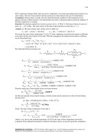
5-88 The passive solar heating of a house through a Trombe wall is studied. The temperature distribution in

the wall in 12 h intervals and the amount of heat transfer during the first and second days are to be
determined.
Assumptions 1 Heat transfer is one-dimensional since the exposed surface of the wall large relative to its
thickness. 2 Thermal conductivity is constant. 3 The heat transfer coefficients are constant.
Properties The wall properties are given to be k = 0.70 W/m⋅°C, α = 0.44 × 10 −6 m 2 /s , and κ = 0.76 . The
hourly variation of monthly average ambient temperature and solar heat flux incident on a vertical surface
is given to be
Time of day
7am-10am
10am-1pm
1pm-4pm
4pm-7pm
7pm-10pm
10pm-1am
1am-4am
4am-7am

Ambient
Temperature, °C
0
4
6
1
-2
-3
-4
-4

Solar insolation
W/m2

375
750
580
95
0
0
0
0

Sun’s
rays

Trombe
wall

hin
Tin

Heat
loss

Heat
gain
hin
Tin

Glazing

Δx
• •

0 1

•
2

• • • •
3 4 5 6

hout
Tout

hout
Tout

Analysis The nodal spacing is given to be Δx = 0.05 m, Then the number of nodes becomes M = L / Δx + 1
= 0.30/0.05+1 = 7. This problem involves 7 unknown nodal temperatures, and thus we need to have 7
equations. Nodes 1, 2, 3, 4, and 5 are interior nodes, and thus for them we can use the general explicit
finite difference relation expressed as
e& mi Δx 2 Tmi +1 − Tmi
→ Tmi +1 = τ (Tmi −1 + Tmi +1 ) + (1 − 2τ )Tmi
=
k
τ
The finite difference equation for boundary nodes 0 and 6 are obtained by applying an energy balance on
the half volume elements and taking the direction of all heat transfers to be towards the node under
consideration:
Tmi −1 − 2Tmi + Tmi +1 +

Node 0: hin A(Tini − T0i ) + kA
or

T1i − T0i
T i +1 − T0i
Δx
= ρA
cp 0
Δx
2
Δt

h Δx
h Δx ⎞
⎛
T0i +1 = ⎜⎜1 − 2τ − 2τ in ⎟⎟T0i + 2τT1i + 2τ in Tini
k
k
⎠
⎝

Node 1 (m = 1) :
Node 2 (m = 2) :

T1i +1 = τ (T0i + T2i ) + (1 − 2τ )T1i
T2i +1 = τ (T1i + T3i ) + (1 − 2τ )T2i

PROPRIETARY MATERIAL. © 2007 The McGraw-Hill Companies, Inc. Limited distribution permitted only to teachers and
educators for course preparation. If you are a student using this Manual, you are using it without permission.


5-73

Node 3 (m = 3) :

T3i +1 = τ (T2i + T4i ) + (1 − 2τ )T3i

Node 4 (m = 4) :

T4i +1 = τ (T3i + T5i ) + (1 − 2τ )T4i

Node 5 (m = 5) :

T5i +1 = τ (T4i + T6i ) + (1 − 2τ )T5i

i
i
hout A(Tout
− T6i ) + κAq& solar
+ kA

Node 6
or

T5i − T6i
T i +1 − T6i
Δx
= ρA
cp 6
Δx
2
Δt

h Δx ⎞
h Δx i
κq& i Δx
⎛
T6i +1 = ⎜⎜1 − 2τ − 2τ out ⎟⎟T6i + 2τT5i + 2τ out Tout
+ 2τ solar
k ⎠
k
k
⎝

where L = 0.30 m, k = 0.70 W/m.°C, α = 0.44 × 10 −6 m 2 /s , Tout and q& solar are as given in the table,
κ = 0.76 hout = 3.4 W/m2.°C, Tin = 20°C, hin = 9.1 W/m2.°C, and Δx = 0.05 m.
Next we need to determine the upper limit of the time step Δt from the stability criteria since we
are using the explicit method. This requires the identification of the smallest primary coefficient in the
system. We know that the boundary nodes are more restrictive than the interior nodes, and thus we
examine the formulations of the boundary nodes 0 and 6 only. The smallest and thus the most restrictive
primary coefficient in this case is the coefficient of T0i in the formulation of node 0 since hin > hout, and
thus
h Δx
h Δx
< 1 − 2τ − 2τ out
1 − 2τ − 2τ in
k
k
Therefore, the stability criteria for this problem can be expressed as

1 − 2τ − 2τ

hin Δx
≥0 →
k

τ≤

1
2(1 + hin Δx / k )

→ Δt ≤

Δx 2
2α (1 + hin Δx / k )

since τ = αΔt / Δx 2 . Substituting the given quantities, the maximum allowable the time step becomes
Δt ≤

(0.05 m) 2
2(0.44 × 10 − 6 m 2 /s)[1 + (9.1 W/m 2 .°C)(0.05 m) /(0.70 W/m.°C)]

= 1722 s

Therefore, any time step less than 1722 s can be used to solve this problem. For convenience, let us choose
the time step to be Δt = 900 s = 15 min. Then the mesh Fourier number becomes

τ=

αΔt
Δx 2

=

(0.44 × 10 −6 m 2 /s)(900 s)
(0.05 m) 2

= 0.1584

Initially (at 7 am or t = 0), the temperature of the wall is said to vary linearly between 20°C at node 0 and
0°C at node 6. Noting that there are 6 nodal spacing of equal length, the temperature change between
two neighboring nodes is (20 - 0)°C/6 = 3.33°C. Therefore, the initial nodal temperatures are

T00 = 20°C, T10 = 16.66°C, T20 = 13.33°C, T30 = 10°C, T40 = 6.66°C, T50 = 3.33°C, T60 = 0°C
Substituting the given and calculated quantities, the nodal temperatures after 6, 12, 18, 24, 30, 36, 42, and
48 h are calculated and presented in the following table and chart.
Time
0 h (7am)
6 h (1 pm)
12 h (7 pm)
18 h (1 am)
24 h (7 am)
30 h (1 pm)
36 h (7 pm)
42 h (1 am)
48 h (7 am)

Time
step, i
0
24
48

72
96
120
144
168
192

Nodal temperatures, °C
T0
T1
T2
20.0
16.7
13.3
17.5
16.1
15.9
21.4
22.9
25.8
22.9
24.6
26.0
21.6
22.5
22.7
21.0
21.8
23.4
24.1

27.0
31.3
24.7
27.6
29.9
23.0
24.6
25.5

T3
10.0
18.1
30.2
26.6
22.1
26.8
36.4
31.1
25.2

T4
6.66
24.8
34.6
26.0
20.4
34.1
41.1
30.5
23.7

T5
3.33
38.8
37.2
23.5
17.7
47.6
43.2
27.8
20.7

T6
0.0
61.5
35.8
19.1
13.9
68.9
40.9
22.6
16.3

PROPRIETARY MATERIAL. © 2007 The McGraw-Hill Companies, Inc. Limited distribution permitted only to teachers and
educators for course preparation. If you are a student using this Manual, you are using it without permission.


5-74

The rate of heat transfer from the Trombe wall to the interior of the house during each time step is

determined from Newton’s law of cooling using the average temperature at the inner surface of the wall
(node 0) as
Qi
= Q& i
Δt = h A(T i − T )Δt = h A[(T i + T i −1) / 2 − T ]Δt
Trumbe wall

Trumbe wall

in

0

in

in

0

0

in

Therefore, the amount of heat transfer during the first time step (i = 1) or during the first 15 min period is
1
1
0
2
2
QTrumbe

wall = hin A[(T0 + T0 ) / 2 − Tin ]Δt = (9.1 W/m .°C)(2.8 × 7 m )[(68.3 + 70) / 2 − 70°C](0.25 h) = −96.8 kWh

The negative sign indicates that heat is transferred to the Trombe wall from the air in the house which
represents a heat loss. Then the total heat transfer during a specified time period is determined by adding
the heat transfer amounts for each time step as
I

QTrumbe wall =

∑Q

i
Trumbe wall

i =1

I

=

∑h

i
in A[(T0

+ T0i −1 ) / 2 − Tin ]Δt

i =1

where I is the total number of time intervals in the specified time period. In this case I = 48 for 12 h, 96 for

24 h, etc. Following the approach described above using a computer, the amount of heat transfer between
the Trombe wall and the interior of the house is determined to be
QTrombe wall = - 3421 kWh after 12 h
QTrombe wall = 1753 kWh after 24 h
QTrombe wall = 5393 kWh after 36 h
QTrombe wall = 15,230 kWh after 48 h
Discussion Note that the interior temperature of the Trombe wall drops in early morning hours, but then
rises as the solar energy absorbed by the exterior surface diffuses through the wall. The exterior surface
temperature of the Trombe wall rises from 0 to 61.5°C in just 6 h because of the solar energy absorbed, but
then drops to 13.9°C by next morning as a result of heat loss at night. Therefore, it may be worthwhile to
cover the outer surface at night to minimize the heat losses.
Also the house loses 3421 kWh through the Trombe wall the 1st daytime as a result of the low
start-up temperature, but delivers about 13,500 kWh of heat to the house the second day. It can be shown
that the Trombe wall will deliver even more heat to the house during the 3rd day since it will start the day
at a higher average temperature.
80
70

Tem perature [C]

60

T0
T1
T2
T3
T4
T5
T6

50
40
30
20
10
0
0

10

20

30

40

50

Tim e [hour]

PROPRIETARY MATERIAL. © 2007 The McGraw-Hill Companies, Inc. Limited distribution permitted only to teachers and
educators for course preparation. If you are a student using this Manual, you are using it without permission.


5-75

5-89 Heat conduction through a long L-shaped solid bar with specified boundary conditions is considered.
The temperature at the top corner (node #3) of the body after 2, 5, and 30 min is to be determined with the
transient explicit finite difference method.
Assumptions 1 Heat transfer through the body is given to be transient and two-dimensional. 2 Thermal

conductivity is constant. 3 Heat generation is uniform.
h, T∞
Properties The conductivity and diffusivity are given to
1
2
be k = 15 W/m⋅°C and α = 3.2 × 10 −6 m 2 /s .
•
•
•3
Analysis The nodal spacing is given to be
qL
Insulated
Δx=Δx=l=0.015 m. The explicit finite difference
4
5
6
7
8
•
•
•
•
•
equations are determined on the basis of the
energy balance for the transient case expressed
as

∑ Q&

i

i
+ E& element
= ρV element c p

All sides

Tmi +1 − Tmi
Δt

140°C

The quantities h, T∞ , e&, and q& R do not change with time, and thus we do not need to use the superscript i
for them. Also, the energy balance expressions can be simplified using the definitions of thermal diffusivity
α = k / ρc p and the dimensionless mesh Fourier number τ = αΔt / l 2 where Δx = Δy = l . We note that all
nodes are boundary nodes except node 5 that is an interior node. Therefore, we will have to rely on energy
balances to obtain the finite difference equations. Using energy balances, the finite difference equations for
each of the 8 nodes are obtained as follows:
Node 1: q& L

l
l
l T2i − T1i
l T4i − T1i
l2
l 2 T1i +1 − T1i
+ h (T∞ − T1i ) + k
+k
+ e& 0
=ρ

c
2
2
2
l
2
l
4
4
Δt

Node 2: hl (T∞ − T2i ) + k
Node 3: hl (T∞ − T3i ) + k

i
i
T i − T2i
T i +1 − T2i
l T1i − T2i
l T3 − T2
l2
l2
+k
+ kl 5
+ e& 0
=ρ
cp 2
2
l
2

l
l
2
2
Δt
i
i
i
i
i +1
i
l T2 − T3
l T6 − T3
l2
l 2 T3 − T3
+k
+ e& 0
=ρ
c
2
l
2
l
4
4
Δt

⎛
e& l 2
hl ⎞

hl
⎛
(It can be rearranged as T3i +1 = ⎜1 − 4τ − 4τ ⎟T3i + 2τ ⎜ T4i + T6i + 2 T∞ + 0
⎜
k ⎠
k
2k
⎝
⎝
Node 4: q& L l + k

⎞
⎟)
⎟
⎠

T i − T4i
l T1i − T4i
l 140 − T4i
l2
l 2 T4i +1 − T4i
+k
+ kl 5
+ e& 0
=ρ
c
2
l
2
l

l
2
2
Δt

⎛
e& l 2
Node 5 (interior): T5i +1 = (1 − 4τ )T5i + τ ⎜ T2i + T4i + T6i + 140 + 0
⎜
k
⎝

⎞
⎟
⎟
⎠

Node 6: hl (T∞ − T6i ) + k

i
i
i
i
i +1
i
T i − T6i
140 − T6i
l T3 − T6
l T7 − T6
3l 2

3l 2 T6 − T6
+ kl 5
+ kl
+k
+ e& 0
=ρ
c
2
l
l
l
2
l
4
4
Δt

Node 7: hl (T∞ − T7i ) + k

i
i
i
i
i +1
i
140 − T7i
l T6 − T7
l T8 − T7
l2
l 2 T7 − T 7

+k
+ kl
+ e& 0
=ρ
c
2
l
2
l
l
2
2
Δt

Node 8: h

i
i
i
i +1
i
l
l T7 − T8
l 140 − T8
l2
l 2 T8 − T8
(T∞ − T8i ) + k
+k
+ e& 0
=ρ

c
2
2
l
2
l
4
4
Δt

where e&0 = 2 × 10 7 W/m 3 , q& L = 8000 W/m 2 , l = 0.015 m, k =15 W/m⋅°C, h = 80 W/m2⋅°C, and T∞
=25°C.

PROPRIETARY MATERIAL. © 2007 The McGraw-Hill Companies, Inc. Limited distribution permitted only to teachers and
educators for course preparation. If you are a student using this Manual, you are using it without permission.


5-76

The upper limit of the time step Δt is determined from the stability criteria that requires the
coefficient of Tmi in the Tmi +1 expression (the primary coefficient) be greater than or equal to zero for all
nodes. The smallest primary coefficient in the 8 equations above is the coefficient of T3i in the T3i +1
expression since it is exposed to most convection per unit volume (this can be verified), and thus the
stability criteria for this problem can be expressed as
1 − 4τ − 4τ

hl
≥0
k

→

τ≤

1
4(1 + hl / k )

→

Δt ≤

l2
4α (1 + hl / k )

since τ = αΔt / l 2 . Substituting the given quantities, the maximum allowable value of the time step is
determined to be
Δt ≤

(0.015 m) 2
4(3.2 × 10 −6 m 2 /s)[1 + (80 W/m 2 .°C)(0.015 m) /(15 W/m.°C)]

= 16.3 s

Therefore, any time step less than 16.3 s can be used to solve this problem. For convenience, we choose the
time step to be Δt = 15 s. Then the mesh Fourier number becomes

τ=

αΔt
l2

=

(3.2 × 10 −6 m 2 /s)(15 s)
(0.015 m) 2

= 0.2133

(for Δt = 15 s)

Using the specified initial condition as the solution at time t = 0 (for i = 0), sweeping through the 9
equations above will give the solution at intervals of 15 s. Using a computer, the solution at the upper
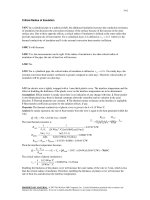
corner node (node 3) is determined to be 441, 520, and 529°C at 2, 5, and 30 min, respectively. It can be
shown that the steady state solution at node 3 is 531°C.

PROPRIETARY MATERIAL. © 2007 The McGraw-Hill Companies, Inc. Limited distribution permitted only to teachers and
educators for course preparation. If you are a student using this Manual, you are using it without permission.


5-77

5-90 EES Prob. 5-89 is reconsidered. The temperature at the top corner as a function of heating time is to
be plotted.
Analysis The problem is solved using EES, and the solution is given below.
"GIVEN"
T_i=140 [C]
k=15 [W/m-C]
alpha=3.2E-6 [m^2/s]
e_dot=2E7 [W/m^3]
T_bottom=140 [C]

T_infinity=25 [C]
h=80 [W/m^2-C]
q_dot_L=8000 [W/m^2]
DELTAx=0.015 [m]
DELTAy=0.015 [m]
time=120 [s]
"ANALYSIS"
l=DELTAx
DELTAt=15 "[s]"
tau=(alpha*DELTAt)/l^2
RhoC=k/alpha "RhoC=rho*C"
"The technique is to store the temperatures in the parametric table and recover them (as old
temperatures)
using the variable ROW. The first row contains the initial values so Solve Table must begin
at row 2.
Use the DUPLICATE statement to reduce the number of equations that need to be typed.
Column 1
contains the time, column 2 the value of T[1], column 3, the value of T[2], etc., and column
10 the Row."
Time=TableValue('Table 1',Row-1,#Time)+DELTAt
Duplicate i=1,8
T_old[i]=TableValue('Table 1',Row-1,#T[i])
end
"Using the explicit finite difference approach, the eight equations for the eight unknown
temperatures are determined to be"
q_dot_L*l/2+h*l/2*(T_infinity-T_old[1])+k*l/2*(T_old[2]-T_old[1])/l+k*l/2*(T_old[4]T_old[1])/l+e_dot*l^2/4=RhoC*l^2/4*(T[1]-T_old[1])/DELTAt "Node 1"
h*l*(T_infinity-T_old[2])+k*l/2*(T_old[1]-T_old[2])/l+k*l/2*(T_old[3]-T_old[2])/l+k*l*(T_old[5]T_old[2])/l+e_dot*l^2/2=RhoC*l^2/2*(T[2]-T_old[2])/DELTAt "Node 2"
h*l*(T_infinity-T_old[3])+k*l/2*(T_old[2]-T_old[3])/l+k*l/2*(T_old[6]T_old[3])/l+e_dot*l^2/4=RhoC*l^2/4*(T[3]-T_old[3])/DELTAt "Node 3"
q_dot_L*l+k*l/2*(T_old[1]-T_old[4])/l+k*l/2*(T_bottom-T_old[4])/l+k*l*(T_old[5]T_old[4])/l+e_dot*l^2/2=RhoC*l^2/2*(T[4]-T_old[4])/DELTAt "Node 4"
T[5]=(1-4*tau)*T_old[5]+tau*(T_old[2]+T_old[4]+T_old[6]+T_bottom+e_dot*l^2/k) "Node 5"

h*l*(T_infinity-T_old[6])+k*l/2*(T_old[3]-T_old[6])/l+k*l*(T_old[5]-T_old[6])/l+k*l*(T_bottomT_old[6])/l+k*l/2*(T_old[7]-T_old[6])/l+e_dot*3/4*l^2=RhoC*3/4*l^2*(T[6]-T_old[6])/DELTAt
"Node 6"
h*l*(T_infinity-T_old[7])+k*l/2*(T_old[6]-T_old[7])/l+k*l/2*(T_old[8]-T_old[7])/l+k*l*(T_bottomT_old[7])/l+e_dot*l^2/2=RhoC*l^2/2*(T[7]-T_old[7])/DELTAt "Node 7"
h*l/2*(T_infinity-T_old[8])+k*l/2*(T_old[7]-T_old[8])/l+k*l/2*(T_bottomT_old[8])/l+e_dot*l^2/4=RhoC*l^2/4*(T[8]-T_old[8])/DELTAt "Node 8"

PROPRIETARY MATERIAL. © 2007 The McGraw-Hill Companies, Inc. Limited distribution permitted only to teachers and
educators for course preparation. If you are a student using this Manual, you are using it without permission.


5-78

Time
[s]
0
15
30
45
60
75
90
105
120
135
…
…
1650
1665
1680
1695
1710

1725
1740
1755
1770
1785

T1 [C]

T2 [C]

T3 [C]

T4 [C]

T5 [C]

T6 [C]

T7 [C]

T8 [C]

Row

140
203.5
265
319
365.5
404.6

437.4
464.7
487.4
506.2
…
…
596.3
596.3
596.3
596.3
596.3
596.3
596.3
596.3
596.3
596.3

140
200.1
259.7
312.7
357.4
394.9
426.1
451.9
473.3
491
…
…
575.7

575.7
575.7
575.7
575.7
575.7
575.7
575.7
575.7
575.7

140
196.1
252.4
300.3
340.3
373.2
400.3
422.5
440.9
456.1
…
…
528.5
528.5
528.5
528.5
528.5
528.5
528.5
528.5

528.5
528.5

140
207.4
258.2
299.9
334.6
363.6
387.8
407.9
424.5
438.4
…
…
504.6
504.6
504.6
504.6
504.6
504.6
504.6
504.6
504.6
504.6

140
204
253.7
293.5

326.4
353.5
375.9
394.5
409.8
422.5
…
…
483.1
483.1
483.1
483.1
483.1
483.1
483.1
483.1
483.1
483.1

140
201.4
243.7
275.7
300.7
320.6
336.7
349.9
360.7
369.6
…

…
411.9
411.9
411.9
411.9
411.9
411.9
411.9
411.9
411.9
411.9

140
200.1
232.7
252.4
265.2
274.1
280.8
286
290.1
293.4
…
…
308.8
308.8
308.8
308.8
308.8
308.8

308.8
308.8
308.8
308.8

140
200.1
232.5
250.1
260.4
267
271.6
275
277.5
279.6
…
…
288.9
288.9
288.9
288.9
288.9
288.9
288.9
288.9
288.9
288.9

1
2

3
4
5
6
7
8
9
10
…
…
111
112
113
114
115
116
117
118
119
120

550
500
450

T 3 [C]

400
350
300

250
200
150
100
0

200

400

600

800 1000 1200 1400 1600 1800

Time [s]

PROPRIETARY MATERIAL. © 2007 The McGraw-Hill Companies, Inc. Limited distribution permitted only to teachers and
educators for course preparation. If you are a student using this Manual, you are using it without permission.


5-79

5-91 A long solid bar is subjected to transient two-dimensional heat transfer. The centerline temperature of
the bar after 20 min and after steady conditions are established are to be determined.
Assumptions 1 Heat transfer through the body is given to be transient and two-dimensional. 2 Heat is
generated uniformly in the body. 3 The heat transfer coefficient also includes the radiation effects.
Properties The conductivity and diffusivity are given to be k = 28
W/m⋅°C and α = 12 × 10 −6 m 2 /s .

h, T∞

Analysis The nodal spacing is given to be Δx=Δx=l=0.1 m. The
explicit finite difference equations are determined on the basis of
the energy balance for the transient case expressed as

∑ Q&

i

i
+ E& element

All sides

1
•

3
•

e

T i +1 − Tmi
= ρV element c p m
Δt

h, T∞ •

4

•

•

7

8
•
h, T∞

The quantities h, T∞ , and e& 0 do not change with time, and thus
we do not need to use the superscript i for them. The general
explicit finite difference form of an interior node for transient twodimensional heat conduction is expressed as
i +1
i
i
i
i
i
= τ (Tleft
+ Ttop
+ Tright
+ Tbottom
) + (1 − 4τ )Tnode
+τ
Tnode

2
•
5

6
• h, T∞
9
•

i
e& node
l2
k

There is symmetry about the vertical, horizontal, and diagonal lines passing through the center. Therefore,
T1 = T3 = T7 = T9 and T2 = T4 = T6 = T8 , and T1 , T2 , and T5 are the only 3 unknown nodal temperatures,
and thus we need only 3 equations to determine them uniquely. Also, we can replace the symmetry lines
by insulation and utilize the mirror-image concept when writing the finite difference equations for the
interior nodes. The finite difference equations for boundary nodes are obtained by applying an energy
balance on the volume elements and taking the direction of all heat transfers to be towards the node under
consideration:
Node 1: hl (T∞ − T1i ) + k
Node 2: h

l T2i − T1i
l T4i − T1i
l2
l 2 T1i +1 − T1i
+k
+ e& 0
=ρ
c
2

l
2
l
4
4
Δt

i
i
l
l T1i − T2i
l T5 − T2
l2
l 2 T2i +1 − T2i
(T∞ − T2i ) + k
+k
+ e& 0
=ρ
c
2
2
l
2
l
4
4
Δt

⎛
e& l 2 ⎞

Node 5 (interior): T5i +1 = (1 − 4τ )T5i + τ ⎜ 4T2i + 0 ⎟
⎜
k ⎟⎠
⎝
where e&0 = 8× 10 5 W/m 3 , l = 0.1 m, and k = 28 W/m⋅°C, h = 45 W/m2⋅°C, and T∞ =30°C.
The upper limit of the time step Δt is determined from the stability criteria that requires the
coefficient of Tmi in the Tmi +1 expression (the primary coefficient) be greater than or equal to zero for all
nodes. The smallest primary coefficient in the 3 equations above is the coefficient of T1i in the T1i +1
expression since it is exposed to most convection per unit volume (this can be verified), and thus the
stability criteria for this problem can be expressed as

1 − 4τ − 4τ

hl
≥0 →
k

τ≤

1
4(1 + hl / k )

→ Δt ≤

l2
4α (1 + hl / k )

since τ = αΔt / l 2 . Substituting the given quantities, the maximum allowable value of the time step is
determined to be
Δt ≤

(0.1 m) 2
4(12 × 10 −6 m 2 /s)[1 + (45 W/m 2 .°C)(0.1 m) /(28 W/m.°C)]

= 179 s

PROPRIETARY MATERIAL. © 2007 The McGraw-Hill Companies, Inc. Limited distribution permitted only to teachers and
educators for course preparation. If you are a student using this Manual, you are using it without permission.


5-80

Therefore, any time step less than 179 s can be used to solve this problem. For convenience, we choose the
time step to be Δt = 60 s. Then the mesh Fourier number becomes

τ=

αΔt
l2

=

(12 × 10 −6 m 2 /s)(60 s)
(0.1 m) 2

= 0.072

(for Δt = 60 s)

Using the specified initial condition as the solution at time t = 0 (for i = 0), sweeping through the 3

equations above will give the solution at intervals of 1 min. Using a computer, the solution at the center
node (node 5) is determined to be 217.2°C, 302.8°C, 379.3°C, 447.7°C, 508.9°C, 612.4°C, 695.1°C, and
761.2°C at 10, 15, 20, 25, 30, 40, 50, and 60 min, respectively. Continuing in this manner, it is observed
that steady conditions are reached in the medium after about 6 hours for which the temperature at the center
node is 1023°C.

PROPRIETARY MATERIAL. © 2007 The McGraw-Hill Companies, Inc. Limited distribution permitted only to teachers and
educators for course preparation. If you are a student using this Manual, you are using it without permission.


5-81

5-92E A plain window glass initially at a uniform temperature is subjected to convection on both sides.
The transient finite difference formulation of this problem is to be obtained, and it is to be determined how
long it will take for the fog on the windows to clear up (i.e., for the inner surface temperature of the
window glass to reach 54°F).
Assumptions 1 Heat transfer is one-dimensional since the window is large relative to its thickness. 2
Thermal conductivity is constant. 3 Radiation heat transfer is negligible.
Properties The conductivity and diffusivity are given to be k = 0.48 Btu/h.ft⋅°F and α = 4.2 × 10 −6 ft 2 /s .
Analysis The nodal spacing is given to be Δx = 0.125 in. Then the number of nodes becomes
M = L / Δx + 1 = 0.375/0.125+1 = 4. This problem involves 4 unknown nodal temperatures, and thus we
need to have 4 equations. Nodes 2 and 3 are interior nodes, and thus for them we can use the general
explicit finite difference relation expressed as
e& mi Δx 2 Tmi +1 − Tmi
→ Tmi +1 = τ (Tmi −1 + Tmi +1 ) + (1 − 2τ )Tmi
=
k
τ
since there is no heat generation. The finite difference equation for nodes 1 and 4 on the surfaces subjected
to convection is obtained by applying an energy balance on the half volume element about the node, and

taking the direction of all heat transfers to be towards the node under consideration:
Tmi −1 − 2Tmi + Tmi +1 +

T2i − T1i
T i +1 − T1i
Δx
cp 1
=ρ
Δx
Δt
2
h Δx ⎞
h Δx
⎛
= ⎜⎜1 − 2τ − 2τ i ⎟⎟T1i + 2τT2i + 2τ i Ti
k
k
⎠
⎝

Node 1 (convection) : hi (Ti − T1i ) + k
or

T1i +1

Node 2 (interior) :

T2i +1 = τ (T1i + T3i ) + (1 − 2τ )T2i

Node 3 (interior) :

T3i +1

Node 4 (convection) :
or

+ T4i ) + (1 − 2τ )T3i
T i − T4i
ho (To − T4i ) + k 3
=ρ

hi
Ti

= τ (T2i

Δx

i +1
i
Δx T4 − T4
c
2
Δt

h Δx ⎞
h Δx
⎛
T4i +1 = ⎜⎜1 − 2τ − 2τ o ⎟⎟T4i + 2τT3i + 2τ o To
k ⎠

k
⎝

Window
glass
ho
To

Δx
•
1

•
2

•
3

4

Fog

where Δx = 0.125/12 ft , k = 0.48 Btu/h.ft⋅°F, hi = 1.2 Btu/h.ft2⋅°F, Ti =35+2*(t/60)°F (t in seconds), ho =
2.6 Btu/h.ft2⋅°F, and To =35°F. The upper limit of the time step Δt is determined from the stability criteria
that requires all primary coefficients to be greater than or equal to zero. The coefficient of T4i is smaller
in this case, and thus the stability criteria for this problem can be expressed as

1 − 2τ − 2τ

hΔx

≥0 →
k

τ≤

1
2(1 + hΔx / k )

→ Δt ≤

Δx 2
2α (1 + hΔx / k )

since τ = αΔt / Δx 2 . Substituting the given quantities, the maximum allowable time step becomes
Δt ≤

(0.125 / 12 ft ) 2
2(4.2 ×10 −6 ft 2 /s)[1 + (2.6 Btu/h.ft 2 .°F)(0.125 / 12 m) /(0.48 Btu/h.ft.°F)]

= 12.2 s

Therefore, any time step less than 12.2 s can be used to solve this problem. For convenience, let us choose
the time step to be Δt = 10 s. Then the mesh Fourier number becomes

τ=

αΔt
Δx 2

=

(4.2 × 10 −6 ft 2 /s)(10 s)
(0.125 / 12 ft ) 2

= 0.3871

Substituting this value of τ and other given quantities, the time needed for the inner surface temperature of
the window glass to reach 54°F to avoid fogging is determined to be never. This is because steady
conditions are reached in about 156 min, and the inner surface temperature at that time is determined to be
48.0°F. Therefore, the window will be fogged at all times.

PROPRIETARY MATERIAL. © 2007 The McGraw-Hill Companies, Inc. Limited distribution permitted only to teachers and
educators for course preparation. If you are a student using this Manual, you are using it without permission.


5-82

5-93 The formation of fog on the glass surfaces of a car is to be
prevented by attaching electric resistance heaters to the inner
surfaces. The temperature distribution throughout the glass 15
min after the strip heaters are turned on and also when steady
conditions are reached are to be determined using the explicit
method.
Assumptions 1 Heat transfer through the glass is given to be
transient and two-dimensional. 2 Thermal conductivity is constant.
3 There is heat generation only at the inner surface, which will be
treated as prescribed heat flux.

Thermal
symmetry line

•
1

∑ Q&

i

All sides

Tmi +1 − Tmi
i
+ E& gen,
element = ρV element c p
Δt

5

7
•

8

Node 1: hi

Node 2: k

•

6

9

• Outer
surface

•

Glass

0.2 cm
•

•

•
1 cm

•

i
i
i +1
i
Δy T2i − T1i
Δy
Δx Δy T1 − T1
Δx T4 − T1
(Ti − T1i ) + k
= ρc p
+k

2
2
2
2 2
Δt
Δx
Δy

•

•

Thermal
symmetry line

T i − T2i
Δy T2i +1 − T2i
Δy T3i − T2i
Δy T1i − T2i
+ kΔx 5
= ρc p Δx
+k
2
2
2
Δt
Δx
Δy
Δx

Node 3: ho

i
i
i +1
i
Δy T2i − T3i
Δy
Δx Δy T3 − T3
Δx T6 − T3
(To − T3i ) + k
= ρc p
+k
2
2
2
2 2
Δt
Δx
Δy

Node 4: hi Δy (Ti − T4i ) + k
Node 5: kΔy

i
i
i +1
i
i
i

T i − T4i
Δx T4 − T4
Δx T7 − T4
Δx T1 − T4
+ kΔy 5
= ρc p Δy
+k
2
2
2
Δt
Δy
Δx
Δy

T4i − T5i
T i − T5i
T i − T5i
T i − T5i
T i +1 − T5i
+ kΔy 6
+ kΔx 8
+ kΔx 2
= ρc p ΔxΔy 5
Δx
Δx
Δy
Δy
Δt

Node 6: ho Δy (Ti − T6i ) + k
Node 7: 5 W + hi

Node 8: k

•

Heater
10 W/m

We consider only 9 nodes because of symmetry. Note that we do
not have a square mesh in this case, and thus we will have to rely
on energy balances to obtain the finite difference equations. Using
energy balances, the finite difference equations for each of the 9
nodes are obtained as follows:

•
3

Inner 4•
surface

Properties The conductivity and diffusivity are given to be
k = 0.84 W/m⋅°C and α = 0.39 × 10 −6 m 2 /s .
Analysis The nodal spacing is given to be Δx = 0.2 cm and Δy = 1
cm. The explicit finite difference equations are determined on the
basis of the energy balance for the transient case expressed as

•
2

i
i
i
i
i +1
i
T i − T6i
Δx T6 − T6
Δx T9 − T6
Δx T3 − T6
+ kΔy 5
= ρc p Δy
+k
2
2
2
Δt
Δy
Δx
Δy

i
i
i +1
i
Δy T8i − T7i
Δy
Δx Δy T7 − T7
Δx T4 − T7

(Ti − T7i ) + k
= ρc p
+k
2
2
2
2 2
Δt
Δx
Δy

T i − T8i
Δy T8i +1 − T8i
Δy T9i − T8i
Δy T7i − T8i
+ kΔx 5
= ρc p Δx
+k
2
2
2
Δt
Δx
Δy
Δx

Node 9: ho

i
i

i +1
i
Δy T8i − T9i
Δy
Δx Δy T9 − T9
Δx T6 − T9
(To − T9i ) + k
= ρc p
+k
2
2
2
2 2
Δt
Δx
Δy

PROPRIETARY MATERIAL. © 2007 The McGraw-Hill Companies, Inc. Limited distribution permitted only to teachers and
educators for course preparation. If you are a student using this Manual, you are using it without permission.


5-83

where k = 0.84 W/m.°C, α = k / ρc = 0.39 ×10 −6 m 2 /s , Ti = To = -3°C hi = 6 W/m2.°C, ho = 20 W/m2.°C,
Δx = 0.002 m, and Δy = 0.01 m.
The upper limit of the time step Δt is determined from the stability criteria that requires the
coefficient of Tmi in the Tmi +1 expression (the primary coefficient) be greater than or equal to zero for all
nodes. The smallest primary coefficient in the 9 equations above is the coefficient of T6i in the T6i +1
expression since it is exposed to most convection per unit volume (this can be verified). The equation for
node 6 can be rearranged as

⎡
⎛ h
1
1
T6i +1 = ⎢1 − 2αΔt ⎜ o + 2 + 2
⎜
Δx
⎢⎣
⎝ kΔx Δy

⎛ h
⎞⎤ i
T i + T9i
T5i
⎟⎥T6 + 2αΔt ⎜ o T0 + 3
+
⎟⎥
⎜ kΔx
Δy 2
Δx 2
⎠⎦
⎝

⎞
⎟
⎟
⎠

Therefore, the stability criteria for this problem can be expressed as
⎛ h

1
1
1 − 2αΔt ⎜ o + 2 + 2
⎜ kΔx Δy
Δx
⎝

⎞
⎟ ≥ 0 → Δt ≤
⎟
⎠

1
⎛ h
1
1
2α ⎜ o + 2 + 2
⎜ kΔx Δy
Δx
⎝

⎞
⎟
⎟
⎠

Substituting the given quantities, the maximum allowable value of the time step is determined to be
or,

Δt ≤

1
⎛
20 W/m ⋅ °C
1
1
2 × (0.39 × 10 m / s )⎜
+
+
⎜ (0.84 W/m ⋅ °C)(0.002 m) (0.002 m) 2 (0.01 m) 2
⎝
2

6

2

⎞
⎟
⎟
⎠

= 4.7 s

Therefore, any time step less than 4.8 s can be used to solve this problem. For convenience, we choose the
time step to be Δt = 4 s. Then the temperature distribution throughout the glass 15 min after the strip
heaters are turned on and when steady conditions are reached are determined to be (from the EES solutions
in CD)
15 min:

T1 = -2.4°C, T2 = -2.4°C, T3 = -2.5°C, T4 = -1.8°C, T5 = -2.0°C,
T6 = -2.7°C, T7 = 12.3°C, T8 = 10.7°C, T9 = 9.6°C

Steady-state:

T1 = -2.4°C, T2 = -2.4°C, T3 = -2.5°C, T4 = -1.8°C, T5 = -2.0°C,
T6 = -2.7°C, T7 = 12.3°C, T8 = 10.7°C, T9 = 9.6°C

Discussion Steady operating conditions are reached in about 8 min.

PROPRIETARY MATERIAL. © 2007 The McGraw-Hill Companies, Inc. Limited distribution permitted only to teachers and
educators for course preparation. If you are a student using this Manual, you are using it without permission.


5-84

5-94 The formation of fog on the glass surfaces of a car is to be
prevented by attaching electric resistance heaters to the inner
surfaces. The temperature distribution throughout the glass 15 min
after the strip heaters are turned on and also when steady
conditions are reached are to be determined using the implicit
method with a time step of Δt = 1 min.
Assumptions 1 Heat transfer through the glass is given to be
transient and two-dimensional. 2 Thermal conductivity is constant.
3 There is heat generation only at the inner surface, which will be
treated as prescribed heat flux.
Properties The conductivity and diffusivity are given to be
k = 0.84 W/m⋅°C and α = 0.39 × 10 −6 m 2 /s .
Analysis The nodal spacing is given to be Δx = 0.2 cm and Δy = 1
cm. The implicit finite difference equations are determined on the

basis of the energy balance for the transient case expressed as

∑ Q&

i +1

i +1
+ E& gen,
element

All sides

T i +1 − Tmi
= ρV element c p m
Δt

We consider only 9 nodes because of symmetry. Note that we
do not have a square mesh in this case, and thus we will have
to rely on energy balances to obtain the finite difference
equations. Using energy balances, the finite difference
equations for each of the 9 nodes are obtained as follows:

Node 1: hi

Node 2: k

•
1

Inner 4•

surface
7
•

•
2

•
3

5

•

8
•

Heater
10 W/m

6

• Outer
surface

9
•

Glass

0.2 cm

•

•

•
1 cm

•

•

•

Thermal
symmetry line

i +1
i +1
i +1
i
Δy T2i +1 − T1i +1
Δy
Δx Δy T1 − T1
Δx T4 − T1
(Ti − T1i +1 ) + k
= ρc p
+k
2

2
2
2 2
Δt
Δx
Δy

T i +1 − T2i +1
Δy T2i +1 − T2i
Δy T3i +1 − T2i +1
Δy T1i +1 − T2i +1
+ kΔx 5
= ρc p Δx
+k
2
2
2
Δt
Δx
Δy
Δx

Node 3: ho

i +1
i +1
i +1
i
Δy T2i +1 − T3i +1
Δy

Δx Δy T3 − T3
Δx T6 − T3
(To − T3i +1 ) + k
= ρc p
+k
2
2
2
2 2
Δt
Δx
Δy

N4: hi Δy (Ti − T4i +1 ) + k
Node 5: kΔy

i +1
i +1
i +1
i
i +1
i +1
T i +1 − T4i +1
Δx T4 − T4
Δx T7 − T4
Δx T1 − T4
+ kΔy 5
= ρc p Δy
+k
2

2
2
Δt
Δy
Δx
Δy

T4i +1 − T5i +1
T i +1 − T5i +1
T i +1 − T5i +1
T i +1 − T5i +1
T i +1 − T5i
+ kΔy 6
+ kΔx 8
+ kΔx 2
= ρc p ΔxΔy 5
Δx
Δx
Δy
Δy
Δt

N6: ho Δy (Ti − T6i +1 ) + k
Node 7: 5 W + hi

Node 8: k

Thermal
symmetry line

i +1
i +1
i +1
i +1
i +1
i
T i +1 − T6i +1
Δx T6 − T6
Δx T9 − T6
Δx T3 − T6
+ kΔy 5
= ρc p Δy
+k
2
2
2
Δt
Δy
Δx
Δy

i +1
i +1
i +1
i
Δy T8i +1 − T7i +1
Δy
Δx Δy T7 − T7
Δx T4 − T7
(Ti − T7i +1 ) + k

= ρc p
+k
2
2
2
2 2
Δt
Δx
Δy

T i +1 − T8i +1
Δy T8i +1 − T8i
Δy T9i +1 − T8i +1
Δy T7i +1 − T8i +1
+ kΔx 5
= ρc p Δx
+k
2
2
2
Δt
Δx
Δy
Δx

Node 9: ho

i +1
i +1
i +1

i
Δy T8i +1 − T9i +1
Δy
Δx Δy T9 − T9
Δx T6 − T9
(To − T9i +1 ) + k
= ρc p
+k
2
2
2
2 2
Δt
Δx
Δy

PROPRIETARY MATERIAL. © 2007 The McGraw-Hill Companies, Inc. Limited distribution permitted only to teachers and
educators for course preparation. If you are a student using this Manual, you are using it without permission.


5-85

where k = 0.84 W/m.°C, α = k / ρc p = 0.39 × 10 −6 m 2 /s , Ti = To = -3°C hi = 6 W/m2.°C, ho = 20 W/m2.°C,
Δx = 0.002 m, and Δy = 0.01 m. Taking time step to be Δt = 1 min, the temperature distribution throughout
the glass 15 min after the strip heaters are turned on and when steady conditions are reached are
determined to be (from the EES solutions in the CD)
15 min:

T1 = -2.4°C, T2 = -2.4°C, T3 = -2.5°C, T4 = -1.8°C, T5 = -2.0°C,
T6 = -2.7°C, T7 = 12.3°C, T8 = 10.7°C, T9 = 9.6°C

Steady-state:

T1 = -2.4°C, T2 = -2.4°C, T3 = -2.5°C, T4 = -1.8°C, T5 = -2.0°C,
T6 = -2.7°C, T7 = 12.3°C, T8 = 10.7°C, T9 = 9.6°C

Discussion Steady operating conditions are reached in about 8 min.

PROPRIETARY MATERIAL. © 2007 The McGraw-Hill Companies, Inc. Limited distribution permitted only to teachers and
educators for course preparation. If you are a student using this Manual, you are using it without permission.


5-86

5-95 The roof of a house initially at a uniform temperature is subjected to convection and radiation on both
sides. The temperatures of the inner and outer surfaces of the roof at 6 am in the morning as well as the
average rate of heat transfer through the roof during that night are to be determined.
Assumptions 1 Heat transfer is one-dimensional. 2 Thermal properties, heat transfer coefficients, and the
indoor and outdoor temperatures are constant. 3 Radiation heat transfer is significant.
Properties The conductivity and diffusivity are given to
be k = 1.4 W/m.°C and α = 0.69 × 10 −6 m 2 /s . The
Tsky
emissivity of both surfaces of the concrete roof is 0.9.
Concrete
Convection
Radiation
Analysis The nodal spacing is given to be Δx = 0.03 m.
roof
h
T

o, o
Then the number of nodes becomes M = L / Δx + 1 =
ε
0.15/0.03+1 = 6. This problem involves 6 unknown
6•
nodal temperatures, and thus we need to have 6
5•
equations. Nodes 2, 3, 4, and 5 are interior nodes, and
4•
thus for them we can use the general explicit finite
3•
difference relation expressed as
2•
e& mi Δx 2 Tmi +1 − Tmi
i
i
i
1•
Tm −1 − 2Tm + Tm +1 +
=
k
τ
ε
Convection
e& mi Δx 2
i +1
i
i
i
Radiation

→ Tm = τ (Tm −1 + Tm +1 ) + (1 − 2τ )Tm + τ
hi, Ti
k
The finite difference equations for nodes 1 and 6 subjected to
convection and radiation are obtained from an energy balance
by taking the direction of all heat transfers to be towards the
node under consideration:
T i − T1i
T i +1 − T1i
Δx
4
Node 1 (convection) : hi (Ti − T1i ) + k 2
+ εσ Twall
− (T1i + 273) 4 = ρ
cp 1
Δx
2
Δt
i +1
i
i
i
Node 2 (interior) :
T2 = τ (T1 + T3 ) + (1 − 2τ )T2

[

Node 3 (interior) :

T3i +1 = τ (T2i + T4i ) + (1 − 2τ )T3i

Node 4 (interior) :

T4i +1 = τ (T3i + T5i ) + (1 − 2τ )T4i

Node 5 (interior) :

T5i +1 = τ (T4i + T6i ) + (1 − 2τ )T5i

]

[

]

T5i − T6i
T i +1 − T6i
Δx
4
+ εσ Tsky
− (T6i + 273) 4 = ρ
cp 6
Δx
2
Δt
−6
2
where k = 1.4 W/m.°C, α = k / ρc p = 0.69 × 10 m /s , Ti = 20°C, Twall = 293 K, To = 6°C, Tsky =260 K,
Node 6 (convection) :

ho (T0 − T6i ) + k

hi = 5 W/m2.°C, ho = 12 W/m2.°C, Δx = 0.03 m, and Δt = 5 min. Also, the mesh Fourier number is
αΔt (0.69 × 10 −6 m 2 /s)(300 s)
= 0.230
τ= 2 =
Δx
(0.03 m) 2
Substituting this value of τ and other given quantities, the inner and outer surface temperatures of the roof
after 12×(60/5) = 144 time steps (12 h) are determined to be T1 = 10.3°C and T6 = -0.97°C.
(b) The average temperature of the inner surface of the roof can be taken to be
T1 @ 6 PM + T1 @ 6 AM 18 + 10.3
T1,avg =
=
= 14.15°C
2
2
Then the average rate of heat loss through the roof that night becomes
) + εσA T 4 − (T i + 273) 4
= h A (T − T
Q&
avg

i

s

i

1, ave

s

[

wall

1

]

= (5 W/m 2 ⋅ °C)(18 × 32 m 2 )(20 - 14.15)°C
+ 0.9(18 × 32 m 2 )(5.67 × 10 -8 W/m 2 ⋅ K 4 )[(293 K) 4 − (14.15 + 273 K) 4 ]
= 33,640 W

PROPRIETARY MATERIAL. © 2007 The McGraw-Hill Companies, Inc. Limited distribution permitted only to teachers and
educators for course preparation. If you are a student using this Manual, you are using it without permission.


5-87

5-96 A refrigerator whose walls are constructed of 3-cm thick urethane insulation malfunctions, and stops
running for 6 h. The temperature inside the refrigerator at the end of this 6 h period is to be determined.
Assumptions 1 Heat transfer is one-dimensional since the walls are large relative to their thickness. 2
Thermal properties, heat transfer coefficients, and the outdoor temperature are constant. 3 Radiation heat
transfer is negligible. 4 The temperature of the contents of the refrigerator, including the air inside, rises
uniformly during this period. 5 The local atmospheric pressure is 1 atm. 6 The space occupied by food and
the corner effects are negligible. 7 Heat transfer through the bottom surface of the refrigerator is negligible.
Properties The conductivity and diffusivity are given to be
k = 0.026 W/m.°C and α = 0.36 × 10 −6 m 2 /s . The average

specific heat of food items is given to be 3.6 kJ/kg.°C. The
Refrigerator
specific heat and density of air at 1 atm and 3°C are cp =
h
o
wall
hi
1.006 kJ/kg.°C and ρ = 1.28 kg/m3 (Table A-15).
To
Ti
Δx
Analysis The nodal spacing is given to be Δx = 0.01
m. Then the number of nodes becomes
•
•
•
•
•
M = L / Δx + 1 = 0.03/0.01+1 = 4. This problem
1
2
3
4
5
involves 4 unknown nodal temperatures, and thus
we need to have 4 equations. Nodes 2 and 3 are
interior nodes, and thus for them we can use the
general explicit finite difference relation expressed
as
e& mi Δx 2 Tmi +1 − Tmi

e& i Δx 2
→ Tmi +1 = τ (Tmi −1 + Tmi +1 ) + (1 − 2τ )Tmi + τ m
=
k
τ
k
The finite difference equations for nodes 1 and 4 subjected to convection and radiation are obtained from
an energy balance by taking the direction of all heat transfers to be towards the node under consideration:
Tmi −1 − 2Tmi + Tmi +1 +

Node 1 (convection) :

T2i − T1i
T i +1 − T1i
Δx
=ρ
cp 1
Δx
2
Δt
i
i
i
= τ (T1 + T3 ) + (1 − 2τ )T2

ho (T0 − T1i ) + k

Node 2 (interior) :

T2i +1

Node 3 (interior) :

T3i +1 = τ (T2i + T4i ) + (1 − 2τ )T3i

T3i − T4i
T i +1 − T4i
Δx
=ρ
cp 4
Δx
2
Δt
2
2
where T5 =Ti = 3°C (initially), To = 25°C, hi = 6 W/m .°C, ho = 9 W/m .°C, Δx = 0.01 m, and Δt = 1 min.
Also, the mesh Fourier number is
Node 4 (convection) :

τ=

αΔt
Δx 2

=

hi (T5i − T4i ) + k

(0.36 × 10 −6 m 2 /s)(60 s)
(0.01 m) 2

= 0.216

The volume of the refrigerator cavity and the mass of air inside are

V = (1.80 − 0.03)(0.8 − 0.03)(0.7 − 0.03) = 0.913 m 3
m air = ρV = (1.28 kg/m 3 )(0.913 m 3 ) = 1.17 kg
Energy balance for the air space of the refrigerator can be expressed as
Node 5 (refrig. air) :
or

where

hi Ai (T4i − T5i ) = (mc p ΔT ) air + (mc p ΔT ) food

[

hi Ai (T4i − T5i ) = (mc p ) air + (mc p ) food

i +1

] T5

− T5i
Δt

Ai = 2 (1 .77 × 0 .77 ) + 2 (1 .77 × 0 .67 ) + ( 0 .77 × 0 .67 ) = 5 .6135 m 2

Substituting, temperatures of the refrigerated space after 6×60 = 360 time steps (6 h) is determined to be
Tin = T5 = 19.6°C

PROPRIETARY MATERIAL. © 2007 The McGraw-Hill Companies, Inc. Limited distribution permitted only to teachers and
educators for course preparation. If you are a student using this Manual, you are using it without permission.


5-88

5-97 EES Prob. 5-96 is reconsidered. The temperature inside the refrigerator as a function of heating time
is to be plotted.
Analysis The problem is solved using EES, and the solution is given below.
"GIVEN"
t_ins=0.03 [m]
k=0.026 [W/m-C]
alpha=0.36E-6 [m^2/s]
T_i=3 [C]
h_i=6 [W/m^2-C]
h_o=9 [W/m^2-C]
T_infinity=25 [C]
m_food=15 [kg]
C_food=3600 [J/kg-C]
DELTAx=0.01 [m]
DELTAt=60 [s]
time=6*3600 [s]
"PROPERTIES"
rho_air=density(air, T=T_i, P=101.3)
C_air=CP(air, T=T_i)*Convert(kJ/kg-C, J/kg-C)
"ANALYSIS"
M=t_ins/DELTAx+1 "Number of nodes"
tau=(alpha*DELTAt)/DELTAx^2
RhoC=k/alpha "RhoC=rho*C"

"The technique is to store the temperatures in the parametric table and recover them (as old
temperatures)
using the variable ROW. The first row contains the initial values so Solve Table must begin
at row 2.
Use the DUPLICATE statement to reduce the number of equations that need to be typed.
Column 1
contains the time, column 2 the value of T[1], column 3, the value of T[2], etc., and column 7
the Row."
Time=TableValue('Table 1',Row-1,#Time)+DELTAt
Duplicate i=1,5
T_old[i]=TableValue('Table 1',Row-1,#T[i])
end
"Using the explicit finite difference approach, the six equations for the six unknown
temperatures are determined to be"
h_o*(T_infinity-T_old[1])+k*(T_old[2]-T_old[1])/DELTAx=RhoC*DELTAx/2*(T[1]T_old[1])/DELTAt "Node 1, convection"
T[2]=tau*(T_old[1]+T_old[3])+(1-2*tau)*T_old[2] "Node 2"
T[3]=tau*(T_old[2]+T_old[4])+(1-2*tau)*T_old[3] "Node 3"
h_i*(T_old[5]-T_old[4])+k*(T_old[3]-T_old[4])/DELTAx=RhoC*DELTAx/2*(T[4]T_old[4])/DELTAt "Node 4, convection"
h_i*A_i*(T_old[4]-T_old[5])=m_air*C_air*(T[5]-T_old[5])/DELTAt+m_food*C_food*(T[5]T_old[5])/DELTAt "Node 5, refrig. air"
A_i=2*(1.8-0.03)*(0.8-0.03)+2*(1.8-0.03)*(0.7-0.03)+(0.8-0.03)*(0.7-0.03)
m_air=rho_air*V_air
V_air=(1.8-0.03)*(0.8-0.03)*(0.7-0.03)

PROPRIETARY MATERIAL. © 2007 The McGraw-Hill Companies, Inc. Limited distribution permitted only to teachers and
educators for course preparation. If you are a student using this Manual, you are using it without permission.


5-89

Time [s]

0
60
120
180
240
300
360
420
480
540
…
…
35460
35520
35580
35640
35700
35760
35820
35880
35940
36000

T1 [C]
3
35.9
5.389
36.75
6.563
37

7.374
37.04
8.021
36.97
…
…
24.85
24.81
24.85
24.81
24.85
24.81
24.85
24.81
24.85
24.82

T2 [C]
3
3
10.11
7.552
13.21
9.968
15.04
11.55
16.27
12.67
…
…

24.23
24.24
24.23
24.24
24.24
24.25
24.25
24.26
24.25
24.26

T3 [C]
3
3
3
4.535
4.855
6.402
6.549
7.891
7.847
8.998
…
…
23.65
23.65
23.66
23.67
23.67
23.68

23.68
23.69
23.69
23.7

T4 [C]
3
3
3
3
3.663
3.517
4.272
4.03
4.758
4.461
…
…
23.09
23.1
23.11
23.12
23.12
23.13
23.14
23.15
23.15
23.16

T5 [C]

3
3
3
3
3
3.024
3.042
3.087
3.122
3.182
…
…
22.86
22.87
22.88
22.88
22.89
22.9
22.91
22.92
22.93
22.94

Row
1
2
3
4
5
6

7
8
9
10
…
…
592
593
594
595
596
597
598
599
600
601

25

20.5

T 5 [C]

16

11.5

7

2.5

0

5000 10000 15000 20000 25000 30000 35000 40000

Tim e [s]

PROPRIETARY MATERIAL. © 2007 The McGraw-Hill Companies, Inc. Limited distribution permitted only to teachers and
educators for course preparation. If you are a student using this Manual, you are using it without permission.


5-90

Special Topic: Controlling the Numerical Error
5-98C The results obtained using a numerical method differ from the exact results obtained analytically
because the results obtained by a numerical method are approximate. The difference between a numerical
solution and the exact solution (the error) is primarily due to two sources: The discretization error (also
called the truncation or formulation error) which is caused by the approximations used in the formulation
of the numerical method, and the round-off error which is caused by the computers' representing a number
by using a limited number of significant digits and continuously rounding (or chopping) off the digits it
cannot retain.
5-99C The discretization error (also called the truncation or formulation error) is due to replacing the
derivatives by differences in each step, or replacing the actual temperature distribution between two
adjacent nodes by a straight line segment. The difference between the two solutions at each time step is
called the local discretization error. The total discretization error at any step is called the global or
accumulated discretization error. The local and global discretization errors are identical for the first time
step.
5-100C Yes, the global (accumulated) discretization error be less than the local error during a step. The
global discretization error usually increases with increasing number of steps, but the opposite may occur
when the solution function changes direction frequently, giving rise to local discretization errors of
opposite signs which tend to cancel each other.

5-101C The Taylor series expansion of the temperature at a specified nodal point m about time ti is
T ( x m , t i + Δt ) = T ( x m , t i ) + Δt

∂T ( x m , t i ) 1 2 ∂ 2 T ( x m , t i )
+ Δt
+L
2
∂t
∂t 2

The finite difference formulation of the time derivative at the same nodal point is expressed as
∂T ( xm , ti ) T ( xm , ti + Δt ) − T ( xm , ti ) Tmi +1 − Tmi
∂T ( xm , ti )
or T ( xm , ti + Δt ) ≅ T ( xm , ti ) + Δt
≅
=
∂t
Δt
Δt
∂t

which resembles the Taylor series expansion terminated after the first two terms.

PROPRIETARY MATERIAL. © 2007 The McGraw-Hill Companies, Inc. Limited distribution permitted only to teachers and
educators for course preparation. If you are a student using this Manual, you are using it without permission.


5-91

5-102C The Taylor series expansion of the temperature at a specified nodal point m about time ti is

T ( x m , t i + Δt ) = T ( x m , t i ) + Δ t

∂T ( x m , t i ) 1 2 ∂ 2 T ( x m , t i )
+ Δt
+L
∂t
2
∂t 2

The finite difference formulation of the time derivative at the same nodal point is expressed as
∂T ( xm , ti ) T ( xm , ti + Δt ) − T ( xm , ti ) Tmi +1 − Tmi
∂T ( xm , ti )
or T ( xm , ti + Δt ) ≅ T ( xm , ti ) + Δt
≅
=
∂t
Δt
Δt
∂t

which resembles the Taylor series expansion terminated after the first two terms. Therefore, the 3rd and
following terms in the Taylor series expansion represent the error involved in the finite difference
approximation. For a sufficiently small time step, these terms decay rapidly as the order of derivative
increases, and their contributions become smaller and smaller. The first term neglected in the Taylor series
expansion is proportional to (Δt ) 2 , and thus the local discretization error is also proportional to (Δt ) 2 .
The global discretization error is proportional to the step size to Δt itself since, at the worst case,
the accumulated discretization error after I time steps during a time period t 0 is

IΔt 2 = (t 0 / Δt )Δt 2 = t 0 Δt which is proportional to Δt.
5-103C The round-off error is caused by retaining a limited number of digits during calculations. It

depends on the number of calculations, the method of rounding off, the type of the computer, and even the
sequence of calculations. Calculations that involve the alternate addition of small and large numbers are
most susceptible to round-off error.
5-104C As the step size is decreased, the discretization error decreases but the round-off error increases.
5-105C The round-off error can be reduced by avoiding extremely small mess sizes (smaller than
necessary to keep the discretization error in check) and sequencing the terms in the program such that the
addition of small and large numbers is avoided.
5-106C A practical way of checking if the round-off error has been significant in calculations is to repeat
the calculations using double precision holding the mesh size and the size of the time step constant. If the
changes are not significant, we conclude that the round-off error is not a problem.
5-107C A practical way of checking if the discretization error has been significant in calculations is to start
the calculations with a reasonable mesh size Δx (and time step size Δt for transient problems), based on
experience, and then to repeat the calculations using a mesh size of Δx/2. If the results obtained by halving
the mesh size do not differ significantly from the results obtained with the full mesh size, we conclude that
the discretization error is at an acceptable level.

PROPRIETARY MATERIAL. © 2007 The McGraw-Hill Companies, Inc. Limited distribution permitted only to teachers and
educators for course preparation. If you are a student using this Manual, you are using it without permission.


5-92

Review Problems

5-108 Starting with an energy balance on a volume
element, the steady three-dimensional finite difference
equation for a general interior node in rectangular
coordinates for T(x, y, z) for the case of constant thermal
conductivity and uniform heat generation is to be obtained.

• n+1
eΔxΔyΔz

Analysis We consider a volume element of size
r •
Δx × Δy × Δz centered about a general interior node (m, n, r)
in a region in which heat is generated at a constant rate of
e& 0 and the thermal conductivity k is variable. Assuming the
m-1 •
direction of heat conduction to be towards the node under
consideration at all surfaces, the energy balance on the
volume element can be expressed as

• m+1

e0
Δy

• r+1

Δx
Δz

•n

ΔE element
Q& cond, left + Q& cond, top + Q& cond, right + Q& cond, bottom + Q& cond, front + Q& cond, back + E& gen,element =
=0
Δt

for the steady case. Again assuming the temperatures between the adjacent nodes to vary linearly, the
energy balance relation above becomes
k (Δy × Δz )

Tm −1,n,r − Tm,n,r

+ k (Δy × Δz )
+ k (Δx × Δy )

+ k (Δx × Δz )

Δx
Tm +1, n,r − Tm, n, r

Δx
Tm, n, r −1 − Tm, n, r
Δz

Tm,n +1,r − Tm, n, r

+ k (Δx × Δz )
+ k (Δx × Δy )

Δy
Tm,n −1,r − Tm, n, r
Δy
Tm,n,r +1 − Tm, n, r
Δz

+ e& 0 (Δx × Δy × Δz ) = 0

Dividing each term by k Δx × Δy × Δz and simplifying gives
Tm −1, n, r − 2Tm, n, r + Tm +1, n, r
Δx

2

+

Tm, n −1, r − 2Tm, n, r + Tm, n +1, r
Δy

2

+

Tm, n, r −1 − 2Tm, n, r + Tm, n, r +1
Δz

2

+

e&0
=0
k

For a cubic mesh with Δx = Δy = Δz = l, and the relation above simplifies to
Tm −1, n, r + Tm +1, n, r + Tm, n −1, r + Tm, n −1, r + Tm, n, r −1 + Tm, n, r +1 − 6Tm, n, r +

e& 0 l 2
=0
k

It can also be expressed in the following easy-to-remember form:
Tleft + Ttop + Tright + Tbottom + Tfront + Tback − 6Tnode +

e& 0 l 2
=0
k

PROPRIETARY MATERIAL. © 2007 The McGraw-Hill Companies, Inc. Limited distribution permitted only to teachers and
educators for course preparation. If you are a student using this Manual, you are using it without permission.