Vibration Simulation using MATLAB and ANSYS App2
Bạn đang xem bản rút gọn của tài liệu. Xem và tải ngay bản đầy đủ của tài liệu tại đây (149.48 KB, 9 trang )
APPENDIX 2
LAPLACE TRANSFORMS
This appendix presents a short introduction to Laplace transforms, the basic
tool used in analyzing continuous systems in the frequency domain. The
Laplace transform converts linear ordinary differential equations (LODE’s)
into algebraic equations, making them easy to solve for their frequency and
time-domain behavior. There are many excellent presentations of the Laplace
transform, as in Oppenheim [1997], for those who would like more
information.
A2.1 Definitions
The Laplace transform is a generalized Fourier transform, where given any
function f(t), the Fourier transform F(ω) is defined as:
∞
F(ω) = F {f (⋅)} (ω) =
∫ f (t) e
j ωt
dt
(A2.1)
−∞
where ω = 2πf and f is frequency, in hz.
In the same spirit, we can define the Laplace transform as:
F(s) = L {f (⋅)} (s) =
+∞
∫ f (t) e
0
− st
dt
(A2.2)
−
where s is complex:
s = σ + jω ,
(A2.3)
σ and ω are real numbers which define the locations of “s” in the complex
plane, see Figure A2.1 below. Also, ω = 2πf as above.
© 2001 by Chapman & Hall/CRC
Im(s)
θ
Re(s)
ωn
ω
σ
Figure A2.1: σ and ω definitions in complex plane.
Remarks:
1) if f (t) ≡ 0 for t < 0 , then
F {f (⋅)} (ω) = L {f (⋅)} ( jω)
(A2.4)
2) The “ 0 − ” limit in the Laplace transform definition takes care of
f (t) 's which contain the δ function.
3) The integral in the definition of the Laplace transform need not be
finite, i.e. L {f } (s) may not exist for all s ∈ . However, if f(t)
is bounded by some exponential:
f (t) ≤ M eσ0 t
then L {f } (s) will make sense for s ∈
© 2001 by Chapman & Hall/CRC
(A2.5)
such that Re {s} > σ0 .
4) The Laplace transform is linear:
L {a1f1 + a 2 f 2 } = a1L {f1 } + a 2 L {f 2 }
(A2.6)
A2.2 Examples, Laplace Transform Table
1) Exponential
f (t) = e − at 1(t)
F(s) =
∞
∞
0−
0−
− at
− st
∫ e 1(t)e dt =
∫e
− (s + a )t
dt =
1
s+a
[s > a ]
(A2.7a,b)
2) Impulse
f (t) = δ(t)
F(s) =
∞
∫ δ(t)e
− st
[for any s ]
dt = e−0 = 1
0−
(A2.8a,b)
3) Step
f (t) = 1(t)
F(s) =
∞
− st
∫ e dt =
0−
− e − s( ∞ ) − e − s(0)
s
=
1
s
[s > 0 ]
(A2.9a,b)
Table A2.1 below contains Laplace transforms for a few selected functions in
the time domain. The “Region of Convergence” or “ROC” is defined as the
range of values of “s” for which the integral in the definition of the Laplace
transform (A2.2) converges (Oppenheim 1997).
© 2001 by Chapman & Hall/CRC
f(t)
Laplace Transform
Region of Convergence
1)
δ(t)
1
all s
2)
δ(t − T)
e − sT
all s
3)
1(t)
1
s
4)
1 m
t 1(t)
m!
5)
e − at 1(t)
1
s+a
Re {s} > Re {a}
6)
1
t m −1e− at 1(t)
(m − 1)!
1
(s + a) m
Re {s} > Re {a}
7)
(1 − e− at )1(t)
a
s(s + a)
8)
(e − at − a − bt )1(t)
9)
sin(at) 1(t)
a
s2 + a 2
Re {s} > 0
10)
cos(at)1(t)
s
s + a2
Re {s} > 0
11)
e − at sin(bt)1(t)
b
(s + a)2 + b 2
Re {s} > a
12)
e − at cos(bt)1(t)
s+a
(s + a)2 + b 2
Re {s} > a
Re {s} > 0
1
s
Re {s} > 0
m +1
b−a
(s + a)(s + b)
Re {s} > max {0, Re {a}}
Re {s} > max {Re {a} , Re {b}}
2
Table A2.1: Laplace transform table.
© 2001 by Chapman & Hall/CRC
A2.3 Duality
The following duality conditions exist:
t f (t) ⇔ −
d
F(s)
ds
(A2.10a,b)
d
f (t) ⇔ s F(s)
dt
A2.4 Differentiation and Integration
Differentiation and the Laplace transform: Suppose
L {x} (s) = X(s)
(A2.11)
then
L {x& } (s) = sX(s) − x(0 − ) ,
(A2.12)
so we can interpret “s” as a differentiation operator:
d
↔s
dt
(A2.13)
Integration and the Laplace transform: Suppose
L {x} (s) = X(s) ,
(A2.14)
t
1
L ∫ x(τ)dτ (s) = X(s) ,
s
0
(A2.15)
then
and we can interpret “1/s” as an integration operator:
t
1
↔ ∫ dt
s
0
© 2001 by Chapman & Hall/CRC
(A2.16)
A2.5 Applying Laplace Transforms to LODE’s with Zero Initial
Conditions
Assume we have a linear ordinary differential equation as shown in (A2.17):
&&&
& + a 3 y(t) = b1&&
& + b3 u(t)
y(t) + a1&&
y(t) + a 2 y(t)
u(t) + b 2 u(t)
(A2.17)
& = 0, y(t) = 0 and take the Laplace transform of both
y(t) = 0, y(t)
Assume &&
sides, using the linearity property (A2.6):
L {&&&
y} (s) + a1L {&&
y} (s) + a 2 L { y& } (s) + a 3 L { y} (s) =
b1L {&&
u} (s) + b 2 L {u& } (s) + b 3 L {u} (s)
(A2.18)
Recalling that “s” is the differentiation operator, replace “dots” with “s”:
s3 Y(s) + a1s 2 Y(s) + a 2 sY(s) + a 3 Y(s) = b1s 2 U(s) + b 2 sU(s) + b 3 U(s) (A2.19)
We are now left with a polynomial equation in “s” that can be factored into
terms multiplying Y(s) and U(s):
s3 + a1s 2 + a 2 s + a 3 Y(s) = b1s 2 + b 2 s + b3 U(s)
(A2.20)
Solving for Y(s):
Y(s) =
b1s 2 + b 2 s + b3
s3 + a1s 2 + a 2 s + a 3
U(s)
(A2.21)
It can be shown that the terms in the numerator and denominator above are the
Laplace transform of the impulse response, H(s):
Y(s) = H(s)U(s) ,
(A2.22)
H(s) = L [ h(⋅) ] (s) ,
(A2.23)
and h(⋅) is the impulse response. For the example LODE (A2.17) the
Laplace transform of the impulse response is:
b1s 2 + b 2 s + b3
H(s) = 3
s + a1s 2 + a 2 s + a 3
© 2001 by Chapman & Hall/CRC
(A2.24)
A2.6 Transfer Function Definition
It can be shown that the transfer function of a system described by a LODE is
the Laplace transform of its impulse response, H(s), (A2.23).
Taking the Laplace transform of the LODE has provided the Laplace
transform of the impulse response. If we could inverse-transform H(s) we
could get the impulse response h(t) without having to integrate the differential
equation. Typically the inverse transform is found by simplifying/expanding
H(s) into terms which can be found in tables, such as Table A2.1, and than
inverting “by inspection.”
A2.7 Frequency Response Definition
Having obtained H(s) directly from the LODE by replacing “dots” by “s,” we
can obtain the frequency response of the system (the Fourier transform of the
impulse response) by substituting “ jω ” for “s” in H(s).
H( jω) = H(s) s = jω
(A2.25)
A2.8 Applying Laplace Transforms to LODE’s with Initial Conditions
In A2.5 we looked at applying Laplace transforms to LODE’s with zero initial
conditions, which led to transfer function and frequency response definitions.
Since transfer functions and frequency responses deal with steady state
sinusoidal excitation response of the system, initial conditions are of no
significance, as it is assumed that all measurements of the system undergoing
sinusoidal excitation are taken over a long enough period of time that
transients have died out.
On the other hand, if we are solving for the transient response of a system
defined by a LODE that has initial conditions, obviously the initial conditions
will not be zero. We will use the basic definition of the differentiation
operation from (A2.12) to define the Laplace transform of 1st and 2nd order
&
differential equations with initial conditions x(0) and x(0)
:
1st Order:
2nd Order:
© 2001 by Chapman & Hall/CRC
& } = sX(s) − x(0)
L {x(t)
&
L {&&
x(t)} = s 2 X(s) − sx(0) − x(0)
(A2.26)
(A2.27)
A2.9 Applying Laplace Transform to State Space
We defined the form of state space equations in Chapter 5 as below:
x& (t) = Ax(t) + Bu(t)
(A2.28)
y (t) = Cx(t) + Du(t)
(A2.29)
where the initial conditions are set by x(0) = xo . The general block diagram
for a SISO state space system is shown in Figure A2.1.
Direct
Transmission
Matrix
D
Integrator Block
Input Matrix
u(t)
B
+
&
x(t)
∫I
Input
Output Matrix
x(t)
C
+
y(t)
Output
System Matrix
scalar
A
vector
Figure A2.1: State space block diagram.
Taking Laplace transform of (A2.28):
L {x& } (s) = L { Ax} (s) + L {Bu} (s)
sX(s) − x(0− ) = AL {x} (s) + BL {u} (s)
(A2.30a,b)
= AX(s) + BU(s)
Solving for X(s):
sX(s) − AX(s) = x(0 − ) + BU(s)
(sI − A ) X(s) = x(0− ) + BU(s)
−1
−
−1
X(s) = (sI − A) x(0 ) + (sI − A ) BU(s)
© 2001 by Chapman & Hall/CRC
(A2.31a,b,c)
The two terms on the right-hand side of (A2.31c) have special significance:
1)
(sI − A )−1 x(0 − ) is the Laplace transform of the homogeneous
solution, the initial condition response.
2)
(sI − A )−1 BU(s) is the Laplace transform of the particular
solution, the forced response.
Taking the Laplace transform of (A2.29), the output equation:
Y (s) = CX(s) + DU(s)
(A2.32)
Knowing X(s) from (A2.31c) and substituting in (A2.32):
Y (s) = C(sI − A )−1 x(0 − ) + C(sI − A )−1 B + D U(s)
(A2.33)
If the initial conditions are zero, x(0 − ) = 0 , then
Y (s) = C(sI − A ) −1 B + D U(s) ,
(A2.34)
with the transfer function for the system being defined by H(s):
H (s) = C(sI − A )−1 B + D
(A2.35)
When the terms in H(s) above are multiplied out, they will result in the
following polynomial form:
H (s) =
© 2001 by Chapman & Hall/CRC
b(s)
+D
a(s)
(A2.36)