Recent advances in robust statistics theory and applications

Claudio Agostinelli · Ayanendranath Basu
Peter Filzmoser · Diganta Mukherjee
Editors

Recent Advances
in Robust
Statistics: Theory
and Applications


Recent Advances in Robust Statistics: Theory
and Applications


Claudio Agostinelli Ayanendranath Basu
Peter Filzmoser Diganta Mukherjee
•

•

Editors

Recent Advances in Robust
Statistics: Theory
and Applications

123


Editors
Claudio Agostinelli

Department of Mathematics
University of Trento
Trento, Italy

Peter Filzmoser
Institute of Statistics and Mathematical
Methods in Economics
Vienna University of Technology
Vienna, Austria

Ayanendranath Basu
Interdisciplinary Statistical Research Unit
Indian Statistical Institute
Kolkata, India

ISBN 978-81-322-3641-2
DOI 10.1007/978-81-322-3643-6

Diganta Mukherjee
Sampling and Official Statistics Unit
Indian Statistical Institute
Kolkata, India

ISBN 978-81-322-3643-6

(eBook)

Library of Congress Control Number: 2016951695
© Springer India 2016
This work is subject to copyright. All rights are reserved by the Publisher, whether the whole or part

of the material is concerned, specifically the rights of translation, reprinting, reuse of illustrations,
recitation, broadcasting, reproduction on microfilms or in any other physical way, and transmission
or information storage and retrieval, electronic adaptation, computer software, or by similar or dissimilar
methodology now known or hereafter developed.
The use of general descriptive names, registered names, trademarks, service marks, etc. in this
publication does not imply, even in the absence of a specific statement, that such names are exempt from
the relevant protective laws and regulations and therefore free for general use.
The publisher, the authors and the editors are safe to assume that the advice and information in this
book are believed to be true and accurate at the date of publication. Neither the publisher nor the
authors or the editors give a warranty, express or implied, with respect to the material contained herein or
for any errors or omissions that may have been made.
Printed on acid-free paper
This Springer imprint is published by Springer Nature
The registered company is Springer (India) Pvt. Ltd.
The registered company address is: 7th Floor, Vijaya Building, 17 Barakhamba Road, New Delhi 110 001, India


Preface

This proceedings volume entitled “Recent Advances in Robust Statistics: Theory
and Applications” outlines the ongoing research in some topics of robust statistics.
It can be considered as an outcome of the International Conference on Robust
Statistics (ICORS) 2015, which was held during January 12–16, 2015, at the Indian
Statistical Institute in Kolkata, India. ICORS 2015 was the 15th conference in this
series, which intends to bring together researchers and practitioners interested in
robust statistics, data analysis and related areas. The ICORS meetings create a
forum to discuss recent progress and emerging ideas in statistics and encourage
informal contacts and discussions among all the participants. They also play an
important role in maintaining a cohesive group of international researchers interested in robust statistics and related topics, whose interactions transcend the
meetings and endure year round. Previously the ICORS meetings were held at the

following places: Vorau, Austria (2001); Vancouver, Canada (2002); Antwerp,
Belgium (2003); Beijing, China (2004); Jyväskylä, Finland (2005); Lisbon,
Portugal (2006); Buenos Aires, Argentina (2007); Antalya, Turkey (2008); Parma,
Italy (2009); Prague, Czech Republic (2010); Valladolid, Spain (2011); Burlington,
USA (2012); St. Petersburg, Russia (2013); and Halle, Germany (2014).
More than 100 participants attended ICORS 2015. The scientific program
included 80 oral presentations. This program had been prepared by the scientific
committee composed of Claudio Agostinelli (Italy), Ayanendranath Basu (India),
Andreas Christmann (Germany), Luisa Fernholz (USA), Peter Filzmoser (Austria),
Ricardo Maronna (Argentina), Diganta Mukherjee (India), and Elvezio Ronchetti
(Switzerland). Aspects of Robust Statistics were covered in the following areas:
robust estimation for high-dimensional data, robust methods for complex data,
robustness based on data depth, robust mixture regression, robustness in functional
data and nonparametrics, statistical inference based on divergence measures, robust
dimension reduction, robust methods in statistical computing, non-standard models
in environmental studies and other miscellaneous topics in robustness.
Taking advantage of the presence of a large number of experts in robust statistics
at the conference, the authorities of the Indian Statistical Institute, Kolkata, and the
conference organizers arranged a one-day pre-conference tutorial on robust
v


vi

Preface

statistics for the students of the institute and other student members of the local
statistics community. Professor Elvezio Ronchetti, Prof. Peter Filzmoser, and
Dr. Valentin Todorov gave the lectures at this tutorial class. All the attendees highly
praised this effort.

All the papers submitted to these proceedings have been anonymously refereed.
We would like to express our sincere gratitude to all the referees. A complete list of
referees is given at the end of the book.
This book contains ten articles which we have organized alphabetically
according to the first author’s name. The paper of Adelchi Azzalini, keynote
speaker at the conference, discusses recent developments in distribution theory as
an approach to robustness. M. Baragilly and B. Chakraborty dedicate their work to
identifying the number of clusters in a data set, and they propose to use multivariate
ranks for this purpose. C. Croux and V. Öllerer use rank correlation measures, like
Spearman’s rank correlation, for robust and sparse estimation of the inverse
covariance matrix. Their approach is particularly useful for high-dimensional data.
The paper of F.Z. Doǧru and O. Arslan examines the mixture regression model,
where robustness is achieved by mixtures of different types of distributions.
A.-L. Kißlinger and W. Stummer propose scaled Bregman distances for the design
of new outlier- and inlier-robust statistical inference tools. A.K. Laha and Pravida
Raja A.C. examine the standardized bias robustness properties of estimators when
the underlying family of distributions has bounded support or bounded parameter
space with applications in circular data analysis and control charts. Large data with
high dimensionality are addressed in the contribution of E. Liski, K. Nordhausen,
H. Oja, and A. Ruiz-Gazen. They use weighted distances between subspaces
resulting from linear dimension reduction methods for combining subspaces of
different dimensions. In their paper, J. Miettinen, K. Nordhausen, S. Taskinen, and
D.E. Tyler focus on computational aspects of symmetrized M-estimators of scatter,
which are multivariate M-estimators of scatter computed on the pairwise differences
of the data. A robust multilevel functional data method is proposed by H.L. Shang
and applied in the context of mortality and life expectancy forecasting. Highly
robust and efficient tests are treated in the contribution of G. Shevlyakov, and the
test stability is introduced as a new indicator of robustness of tests.
We would like to thank all the authors for their work, as well as all referees for
sending their reviews in time.

Trento, Italy
Kolkata, India
Vienna, Austria
Kolkata, India
April 2016

Claudio Agostinelli
Ayanendranath Basu
Peter Filzmoser
Diganta Mukherjee


Contents

Flexible Distributions as an Approach to Robustness:
The Skew-t Case . . . . . . . . . . . . . . . . . . . . . . . . . . . . . . . . . . . . . . . . . . . . .
Adelchi Azzalini
Determining the Number of Clusters Using Multivariate Ranks . . . . . . .
Mohammed Baragilly and Biman Chakraborty

1
17

Robust and Sparse Estimation of the Inverse Covariance
Matrix Using Rank Correlation Measures . . . . . . . . . . . . . . . . . . . . . . . .
Christophe Croux and Viktoria Öllerer

35

Robust Mixture Regression Using Mixture of Different

Distributions . . . . . . . . . . . . . . . . . . . . . . . . . . . . . . . . . . . . . . . . . . . . . . . .
Fatma Zehra Doğru and Olcay Arslan

57

Robust Statistical Engineering by Means of Scaled
Bregman Distances . . . . . . . . . . . . . . . . . . . . . . . . . . . . . . . . . . . . . . . . . . .
Anna-Lena Kißlinger and Wolfgang Stummer

81

SB-Robustness of Estimators . . . . . . . . . . . . . . . . . . . . . . . . . . . . . . . . . . . 115
Arnab Kumar Laha and A.C. Pravida Raja
Combining Linear Dimension Reduction Subspaces . . . . . . . . . . . . . . . . . 131
Eero Liski, Klaus Nordhausen, Hannu Oja and Anne Ruiz-Gazen
On the Computation of Symmetrized M-Estimators of Scatter . . . . . . . . 151
Jari Miettinen, Klaus Nordhausen, Sara Taskinen and David E. Tyler
Mortality and Life Expectancy Forecasting for a Group
of Populations in Developed Countries: A Robust Multilevel
Functional Data Method . . . . . . . . . . . . . . . . . . . . . . . . . . . . . . . . . . . . . . . 169
Han Lin Shang

vii


viii

Contents

Asymptotically Stable Tests with Application to Robust Detection . . . . . 185

Georgy Shevlyakov
List of Referees . . . . . . . . . . . . . . . . . . . . . . . . . . . . . . . . . . . . . . . . . . . . . . 201


About the Editors

Claudio Agostinelli is Associate Professor of Statistics at the Department of
Mathematics, University of Trento, Italy. He received his Ph.D. in Statistics from
the University of Padova, Italy, in 1998. Prior to joining the University of Trento,
he was Associate Professor at the Department of Environmental Sciences,
Informatics and Statistics, Ca’ Foscari University of Venice, Italy. His principal
area of research is robust statistics. He also works on statistical data depth, circular
statistics and computational statistics with applications to paleoclimatology and
environmental sciences. He has published over 35 research articles in international
refereed journals. He is associate editor of Computational Statistics. He is member
of the ICORS steering committee.
Ayanendranath Basu is Professor at the Interdisciplinary Statistical Research
Unit of the Indian Statistical Institute, Kolkata, India. He received his M.Stat. from
the Indian Statistical Institute, Kolkata, in 1986, and his Ph.D. in Statistics from the
Pennsylvania State University in 1991. Prior to joining the Indian Statistical
Institute, Kolkata, he was Assistant Professor at the Department of Mathematics,
University of Texas at Austin, USA. Apart from his primary interest in robust
minimum distance inference, his research areas include applied multivariate analysis, categorical data analysis, statistical computing, and biostatistics. He has
published over 90 research articles in international refereed journals and has
authored and edited several books and book chapters. He is a recipient of the C.R.
Rao National Award in Statistics given by the Government of India. He is a Fellow
of the National Academy of Sciences, India, and the West Bengal Academy of
Science and Technology. He is a past editor of Sankhya, The Indian Journal of
Statistics, Series B.
Peter Filzmoser studied applied mathematics at the Vienna University of

Technology, Austria, where he also wrote his doctoral thesis and habilitation. His
research led him to the area of robust statistics, resulting in many international
collaborations and various scientific papers in this area. He has been involved in
organizing several scientific events devoted to robust statistics, including the first
ICORS conference in 2001 in Austria. Since 2001, he has been Professor at the
ix


x

About the Editors

Department of Statistics at the Vienna University of Technology, Austria. He was
Visiting Professor at the Universities of Vienna, Toulouse, and Minsk. He has
published over 100 research articles, authored five books and edited several proceedings volumes and special issues of scientific journals. He is an elected member
of the International Statistical Institute.
Diganta Mukherjee holds M.Stat. and then Ph.D. (Economics) degrees from the
Indian Statistical Institute, Kolkata. His research interests include welfare and
development economics and finance. Previously he was a faculty in the Jawaharlal
Nehru University, India, Essex University, UK, and the ICFAI Business School,
India. He is now a faculty at the Indian Statistical Institute, Kolkata. He has over 60
publications in national and international journals and has authored three books.
He has been involved in projects with large corporate houses and various ministries
of the Government of India and the West Bengal government. He is acting as a
technical advisor to MCX, RBI, SEBI, NSSO, and NAD (CSO).


Flexible Distributions as an Approach
to Robustness: The Skew-t Case
Adelchi Azzalini

1 Flexible Distributions and Adaptive Tails
1.1 Some Early Proposals
The study of parametric families of distributions with high degree of flexibility,
suitable to fit a wide range of shapes of empirical distributions, has a long-standing
tradition in statistics; for brevity, we shall refer to this context with the phrase ‘flexible
distributions’. An archetypal exemplification is provided by the Pearson system with
its 12 types of distributions, but many others could be mentioned.
Recall that, for non-transition families of the Pearson system as well as in various
other formulations, a specific distribution is identified by four parameters. This allows
us to regulate separately from each other four qualitative aspects of a distribution,
namely location, scale, slant and tail weight. In the context of robust methods, the
appealing aspect of flexibility is represented by the possibility of regulating the tail
weight of a continuous distribution to accommodate outlying observations.
When a continuous variable of interest spans the whole real line, an interesting
distribution is the one with density function
cν exp −

|x|ν
ν

,

x ∈ R,

(1)

where ν > 0 and the normalizing constant is cν = {2 ν 1/ν Γ (1 + 1/ν)}−1 . Here the
parameter ν manoeuvres the tail weight in the sense that ν = 2 corresponds to the
normal distribution, 0 < ν < 2 produces tails heavier than the normal ones, ν > 2

produces lighter tails. The original expression of the density put forward by Subbotin
(1923) was set in a different parameterization, but this does not affect our discussion.
A. Azzalini (B)
Department of Statistical Sciences, University of Padua, Padua, Italy
e-mail:
© Springer India 2016
C. Agostinelli et al. (eds.), Recent Advances in Robust Statistics:
Theory and Applications, DOI 10.1007/978-81-322-3643-6_1

1


2

A. Azzalini

This flexibility of tail weight provides the motivation for Box and Tiao (1962),
Box and Tiao (1973, Sect. 3.2.1), within a Bayesian framework, to adopt the Subbotin’s family of distributions, complemented with a location parameter μ and a
scale parameter σ , as the parametric reference family allows for departure from normality in the tail behaviour. This logic provides a form of robustness in inference on
the parameters of interest, namely μ and σ , since the tail weight parameter adjusts
itself to non-normality of the data. Strictly speaking, they consider only a subset of
the whole family (1), since the role of ν is played by the non-normality parameter β ∈ (−1, 1] whose range corresponds to ν ∈ [1, ∞) and β = 0 corresponds to
ν = 2.
Another formulation with a similar, and even more explicit, logic is the one of
Lange et al. (1989). They work in a multivariate context and the error probability
distribution is taken to be the Student’s t distribution, where the tail weight parameter
ν is constituted by the degrees of freedom. Again the basic distribution is complemented by a location and a scale parameter, which are now represented by a vector
μ and a symmetric positive-definite matrix, possibly parametrized by some lower
dimensional parameter, say ω. Robustness of maximum likelihood estimates (MLEs)
of the parameters of interest, μ and ω, occurs “in the sense that outlying cases with

large Mahalanobis distances […] are downweighted”, as visible from consideration
of the likelihood equations.
The Student’s t family allows departures from normality in the form of heavier tails, but does not allow lighter tails. However, in a robustness context, this is
commonly perceived as a minor limitation, while there is the important advantage
of closure of the family of distributions with respect to marginalization, a property
which does not hold for the multivariate version of Subbotin’s distribution (Kano
1994).
The present paper proceeds in a similar conceptual framework, with two main
aims: (a) to include into consideration also more recent and general proposals of
parametric families, (b) to discuss advantages and disadvantages of this approach
compared to canonical methods of robustness. For simplicity of presentation, we
shall confine our discussion almost entirely to the univariate context, but the same
logic carries on in the multivariate case.

1.2 Flexibility via Perturbation of Symmetry
In more recent years, much work has been devoted to the construction of highly
flexible families of distributions generated by applying a perturbation factor to a
‘base’ symmetric density. More specifically, in the univariate case, a density f 0
symmetric about 0 can be modulated to generate a new density
f (x) = 2 f 0 (x) G 0 {w(x)},

x ∈ R,

(2)


Flexible Distributions as an Approach to Robustness: The Skew-t Case

3

for any odd function w(x) and any continuous distribution function G 0 having density
symmetric about 0. By varying the ingredients w and G 0 , a base density f 0 can
give rise to a multitude of new densities f , typically asymmetric but also of more
varied shapes. A recent comprehensive account of this formulation, inclusive of its
multivariate version, is provided by Azzalini and Capitanio (2014).
One use of mechanism (2) is to introduce asymmetric versions of the Subbotin and
Student’s t distributions via the modulation factor G 0 {w(x)}. Consider specifically
the case when the base density is taken to be the Student’s t on ν degrees of freedom,
that is,
−(ν+1)/2
x2
Γ ((ν + 1)/2)
,
x ∈ R.
(3)
1+
t (x; ν) = √
ν
π ν Γ (ν/2)
In principle, the choice of the factor G 0 {w(x)} is bewildering wide, but there are
reasons for focusing on the density, denoted as skew-t (ST for short),
t (x; α, ν) = 2 t (x; ν) T

αx

ν+1
;ν + 1 ,
ν + x2

(4)

where T (·; ρ) represents the distribution function of a t variate with ρ degrees of
freedom and α ∈ R is a parameter which regulates slant; α = 0 gives back the original
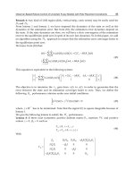
Student’s t. Density (4) is displayed in Fig. 1 for a few values of ν and α.
We indicate only one of the reasons leading to the apparently peculiar final factor
of (4). Start by a continuous random variable Z 0 of skew-normal type, that is, with
density function
ϕ(x; α) = 2 ϕ(x) Φ(α x),
x ∈R
(5)
ν=5

0.6

ν =1

0.6

α=0
α=2
α=5
α = 20

0.0

0.0

0.1

0.2

0.2

t1
0.3

t5
0.4

0.4

0.5

α=0
α=2
α=5
α = 20

−2

−1

0

1

2

3

4

−2

−1

0

1

2

3

4

Fig. 1 Skew-t densities when ν = 1 in the left plot and ν = 5 in the right plot. For each plot,
various values of α are considered with α ≥ 0; the corresponding negative values of α mirror the
curves on the opposite side of the vertical axis


4

A. Azzalini

where ϕ and Φ denote the N(0, 1) density and distribution function. An overview
of this distribution is provided in Chap. 2 of Azzalini and Capitanio (2014). Con√
sider further V ∼ χν2 /ν, independent of Z 0 , and the transformation Z = Z 0 / V ,
traditionally applied with Z 0 ∼ N(0, 1) to obtain the classical t distribution (3). On
assuming instead that Z 0 is of type (5), it can be shown that Z has distribution (4).

For practical work, we introduce location and scale parameters via the transformation Y = ξ + ω Z , leading to a distribution with parameters (ξ, ω, α, ν); in this
case we write
(6)
Y ∼ ST(ξ, ω2 , α, ν) .
Because of asymmetry of Z , here ξ does not coincide with the mean value μ; similarly, ω does not equal the standard deviation σ . Actually, a certain moment exists
only if ν exceeds the order of that moment, like for an ordinary t distribution. Provided ν > 4, there are known expressions connecting (ξ, ω, α, ν) with (μ, σ, γ1 , γ2 ),
where the last two elements denote the third and fourth standardized cumulants,
commonly taken to be the measures of skewness and excess kurtosis. Inspection
of these measures indicates a wide flexibility of the distribution as the parameters
vary; notice however that the distribution can be employed also with ν ≤ 4, and actually low values of ν represent an interesting situation for applications. Mathematical
details omitted here and additional information on the ST distribution are provided
in Sects. 4.3 and 4.4 of Azzalini and Capitanio (2014).
Clearly, expression (2) can also be employed with other base distributions and
another such option is distribution (1), as expounded in Sect. 4.2 of Azzalini and
Capitanio (2014). We do not dwell in this direction because (i) conceptually the
underlying logical frame is the same of the ST distribution and (ii) there is a mild
preference for the ST proposal. One of the reasons for this preference is similar to
the one indicated near the end of Sect. 1.1 in favour of the symmetric t distribution,
which is closed under marginalization in the multivariate case and this fact carries
on for the ST distribution. Azzalini and Genton (2008) and Sect. 4.3.2 of Azzalini
and Capitanio (2014) provide a more extensive discussion of this issue, including
additional arguments.
To avoid confusion, the reader must be aware of the existence of other distributions
named skew-t in the literature. The one considered here was, presumably, the first
construction with this name. The original expression of the density by Branco and Dey
(2001) appeared different, since it was stated in an integral form, but subsequently
proved by Azzalini and Capitanio (2003) to be equivalent to (3).
The high flexibility of these distributions, specifically the possibility to regulate
their tail weight combined with asymmetry, supports their use in the same logic of
the papers recalled in Sect. 1.1. Azzalini (1986) has motivated the introduction of

asymmetric versions of Subbotin distribution precisely by robustness considerations,
although this idea has not been complemented by numerical exploration. Azzalini
and Genton (2008) have worked in a similar logic, but focusing mainly on the ST
distribution as the working reference distribution; more details are given in Sect. 3.4.
To give a first perception of the sort of outcome to be expected, let us consider
a very classical benchmark of robustness methodology, perhaps the most classical:


Flexible Distributions as an Approach to Robustness: The Skew-t Case

5

Table 1 Total absolute deviation of various fitting methods applied to the stack loss data
Method
LS
Huber
LTS
MM
MLE-ST
Q

49.7

46.1

49.4

45.3

43.4

the ‘stack loss’ data. We use the data following the same scheme of many existing
publications, by fitting a linear regression model with the three available explanatory
variables plus intercept to the response variable y, i. e. the stack loss, and examine
the discrepancy between observed and fitted values along the n = 21 data points. A
simple measure of the achieved goodness of fit is represented by the total absolute
deviation
n

|yi − yˆi |,

Q=
i=1

where yi denotes the ith observation of the response variable and yˆi is the corresponding fitted value produced by any candidate method. The methods considered
are the following: least squares (LS, in short), Huber estimator with scale parameter estimated by minimum absolute deviation, least trimmed sum of squares (LTS)
of Rousseeuw and Leroy (1987), MM estimation proposed by Yohai (1987), MLE
under assumption of ST distribution of the error term (MLE-ST). For the ST case,
an adjustment to the intercept must be made to account for the asymmetry of the
distribution; here we have added the median of the fitted ST error distribution to the
crude estimate of the intercept. The outcome is reported in Table 1, whose entries
have appeared in Table 5 of Azzalini and Genton (2008) except that MM estimation
was not considered there. The Q value of MLE-ST is the smallest.

2 Aspects of Robustness
2.1 Robustness and Real Data
The effectiveness of classical robust methods in work with real data has been questioned in a well-known paper by Stigler (1977). In the opening section, the author
lamented that ‘most simulation studies of the robustness of statistical procedures have
concentrated on a rather narrow range of alternatives to normality: independent, identically distributed samples from long-tailed symmetric continuous distributions’ and
proposed instead ‘why not evaluate the performance of statistical procedures with

real data?’ He then examined 24 data sets arising from classical experiments, all
targeted to measure some physical or astronomical quantity, for which the modern
measurement can be regarded as the true value. After studying these data sets, including application of a battery of 11 estimators on each of them, the author concluded
in the final section that ‘the data sets examined do exhibit a slight tendency towards


6

A. Azzalini

more extreme values that one would expect from normal samples, but a very small
amount of trimming seems to be the best way to deal with this. […] The more drastic
modern remedies for feared gross errors […] lead here to an unnecessary loss of
efficiently.’
Similarly, Hill and Dixon (1982) start by remarking that in the robustness literature ‘most estimators have been developed and evaluated for mathematically wellbehaved symmetric distributions with varying degrees of high tail’, while ‘limited
consideration has been given to asymmetric distributions’. Also in this paper the
programme is to examine the distribution of really observed data, in this case originating in an clinical laboratory context, and to evaluate the behaviour of proposed
methods on them. Specifically, the data represent four biomedical variables recorded
on ‘3000 apparently well visitors’ of which, to obtain a fairly homogeneous population, only data from women 20–50 years old were used, leading to sample sizes
in the range 1037–1110 for the four variables. Also for these data, the observed
distributions ‘differ from many of the generated situations currently in vogue: the
tails of the biomedical distributions are not so extreme, and the densities are often
asymmetric, lumpy and have relatively few unique values’. Other interesting aspects
arise by repeatedly extracting subsamples of size 10, 20 and 40 from the full set,
computing various estimators on these subsamples and examining the distributions
of the estimators. The indications that emerge include the fact that the population
values of the robust estimators do not estimate the population mean; moreover, as the
distributions become more asymmetric, the robust estimates approach the population
median, moving away from the mean.
A common indication from the two above-quoted papers is that the observed distributions display some departure from normality, but tail heaviness is not as extreme as

in many simulation studies of the robustness literature. The data display instead other
forms of departures from ideal conditions for classical methods, especially asymmetry and “lumpiness” or granularity. However, the problem of granularity will be
presumably of decreasing importance as technology evolves, since data collection
takes place more and more frequently in an automated manner, without involving
manual transcription and consequent tendency to number rounding, as it was commonly the case in the past.
Clearly, these indications must not be regarded as universal. Stigler (1977, Sect. 6)
himself recognizes that ‘some real data sets with symmetric heavy tails do exist, cannot be denied’. In addition, it can be remarked that the data considered in the quoted
papers are all of experimental or laboratory origin, and possibly in a social sciences
context the picture may be somewhat different. However, at the least, the indication
remains that the distribution of real data sets is not systematically symmetric and
not so heavy tailed as one could perceive from the simulation studies employed in a
number of publications.


Flexible Distributions as an Approach to Robustness: The Skew-t Case

7

2.2 Some Qualitative Considerations
The plan of this section is to discuss qualitatively the advantages and limitation of the
proposed approach, also in the light of the facts recalled in the preceding subsection.
For the sake of completeness, let us state again and even more explicitly the
proposed line of work. For the estimation of parameters of interest in a given inferential problem, typically location and scale, we embed them in a parametric class
which includes some additional parameters capable of regulating the shape and tail
behaviour of the distribution, so to accommodate outlying observations as manifestations of the departures from normality of these distributions, hence providing a
form of robustness. In a regression context, the location parameter is replaced by the
regression parameters as the focus of primary interest.
In this logic, an especially interesting family of distributions is the skew-t, which
allows to regulate both its asymmetry and tail weight, besides location and scale.
Such a usage of the distribution was not the original motivation of its design, which

was targeted to flexibility to adapt itself to a variety of situations, but this flexibility
leads naturally to this other role.
The formulation prompts a number of remarks, in different and even contrasting
directions, partly drawing from Azzalini and Genton (2008) and from Azzalini and
Capitanio (2014, Sect. 4.3.5).
1. Clearly the proposed route does not belong to the canonical formulation of robust
methods, as presented for instance by Huber and Ronchetti (2009), and one cannot expect it to fulfil the criteria stemming from that theory. However, some
connections exist. Hill and Dixon (1982, Sect. 3.1) have noted that the Laszlo
robust estimator of location coincides with the MLE for the location parameter
of a Student’s t when its degrees of freedom are fixed. Lucas (1997), He et al.
(2000) examine this connection in more detail, confirming the good robustness
properties of MLE of the location parameter derived from an assumption of t
distribution with fixed degrees of freedom.
2. The key motivation for adopting the flexible distributions approach is to work with
a fully specified parametric model. Among the implied advantages, an important
one is that it is logically clear what the estimands are: the parameters of the
model. The same question is less transparent with classical robust methods. For
the important family of M-estimators, the estimands are given implicitly as the
solution of a certain nonlinear equation; see for instance Theorem 6.4 of Huber
and Ronchetti (2009). In the simple case of a location parameter estimated using
an odd ψ-function when the underlying distribution is symmetric around a certain
value, the estimand is that centre of symmetry, but in a more general setting we
are unable to make a similarly explicit statement.
3. Another advantage of a fully specified parametric model is that, at the end of the
inference process, we obtain precisely that, a fitted probability model. Hence, as
a simple example, one can assess the probability that a variable of interest lies
in a given interval (a, b), a question which cannot be tackled if one works with
estimating equations as with M-estimates.

8

A. Azzalini

4. The critical point for a parametric model is of course the inclusion of the true
distribution underlying the data generation among those contemplated by the
model. Since models can only approximate reality, this ideal situation cannot be
met exactly in practice, except exceptional situations. If we denote by θ ∈ Θ ⊆
R p the parameter of a certain family of distributions, f (x; θ ), recall that, under
suitable regularity conditions, the MLE θˆ of θ converges in probability to the value
θ0 ∈ Θ such that f (x; θ0 ) has minimal Kullback–Leibler divergence from the true
distribution. The approach via flexible distributions can work satisfactorily insofar
it manages to keep this divergence limited in a wide range of cases.
5. Classical robust methods are instead designed to work under all possible situations, even the most extreme. On the other hand, empirical evidence recalled in
Sect. 2.1 indicates that protection against all possible alternatives may be more
than we need, as in the real world the most extreme situations do not arise that
often.
6. As for the issue discussed in item 4, we are not disarmed, because the adequacy
of a parametric model can be tested a posteriori using model diagnostic tools,
hence providing a safeguard against appreciable Kullback–Leibler divergence.

3 Some Quantitative Indications
The arguments presented in Sect. 2.2, especially in items 4 and 5 of the list there,
call for quantitative examination of how the flexible distribution approach works
in specific cases, especially when the data generating distributions does not belong
to the specified parametric distribution, and how it compares with classical robust
methods.
This is the task of the present section, adopting the ST parametric family (6) and
using MLE for estimation; for brevity we refer to this option as MLE-ST. Notice
that ν is not fixed in advance, but estimated along with the other parameters. When a

similar scheme is adopted for the classical Student’s t distribution, Lucas (1997) has
shown that the influence function becomes unbounded, hence violating the canonical
criteria for robustness. A similar fact can be shown to happen with the ST distribution.

3.1 Limit Behaviour Under a Mixture Distribution
Recall the general result about the limit behaviour of the MLE when a certain parametric assumption is made on the distribution of an observed random variable Y ,
whose actual distribution p(·) may not be a member of the parametric class. Under
the assumption of independent sampling from Y with constant distribution p and
various regularity conditions, Theorem 2 of Huber (1967) states that the MLE of
parameter θ converges almost surely to the solution θ0 , assumed to be unique, of the
equation


9

0.04
0.02

density

0.06

Flexible Distributions as an Approach to Robustness: The Skew-t Case

Huber:proposal2
ST:median

0

0.00

ST:mean

0

5

10

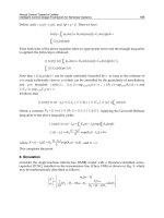
Fig. 2 The shaded area represents the main body of distribution (8) when π = 0.05, Δ = 10,
σ = 3 and the small circle on the horizontal axis marks its mean value; the dashed curve represents
the corresponding MLE-ST limit distribution. The vertical bars denote the estimands of Huber’s
‘proposal 2’ and of MLE-ST, the latter one in two variants, mean value and median

E p {ψ(Y ; θ )} = 0,

(7)

where the subscript p indicates that the expectation is taken with respect to that
distribution and ψ(·; θ ) denotes the score function of the parametric model.
We examine numerically the case where the parametric assumption is of ST type
with θ = (ξ, ω, α, ν) and p(x) represents a contaminated normal distribution, that
is, a mixture density of the form
p(x) = (1 − π ) ϕ(x) + π σ −1 ϕ{σ −1 (x − Δ)} .

(8)

In our numerical work, we have set π = 0.05, Δ = 10, σ = 3. The corresponding p(x) is depicted as a grey-shaded area in Fig. 2 and its mean value, 0.5,
is marked by a small circle on the horizontal axis. The expression of the fourdimensional score function for the ST assumption is given by DiCiccio and Monti
(2011), reproduced with inessential changes of notation in Sect. 4.3.3 of Azzalini and Capitanio (2014). The solution of (7) obtained via numerical methods is

θ0 = (−0.647, 1.023, 1.073, 2.138), whose corresponding ST density is represented
by the dashed curve in Fig. 2. From θ0 , we can compute standard measures of location, such as the mean and the median of the ST distribution with that parameter;
their values, 0.0031 and 0.3547, are marked by vertical bars on the plot. The first of
these values is almost equal to the centre of the main component of p(x), i. e. ϕ(x),
while the mean of the ST distribution is not far from the mean of p(x). Which of the
two quantities is more appropriate to consider depends, at least partly, on the specific
application under consideration.


10

A. Azzalini

To obtain a comparison term from a classical robust technique, a similar numerical
evaluation has been carried out for ‘proposal 2’ of Huber (1964), where θ comprises a
location and a scale parameter. The corresponding estimands are computed solving an
equation formally identical to (7), except that now ψ represents the set of estimating
equations, not the score function; see Theorem 6.4 of Huber and Ronchetti (2009).
For the case under consideration, the location estimand is 0.0957, which is also
marked by a vertical bar in Fig. 2. This value is intermediate to the earlier values of
the ST distribution, somewhat closer to the median, but anyway they are all not far
away from each other.
For the ST distribution, alternative measures of location, scale and so on, which
are formally similar to the corresponding moment-based quantities but exist for all
ν > 0, have been proposed by Arellano-Valle and Azzalini (2013). In the present
case, the location measure of this type, denoted pseudomean, is equal to 0.1633
which is about halfway the ST mean and median; this value is not marked on Fig. 2
to avoid cluttering.

3.2 A Non-random Simulation

We examine the behaviour of ST-MLE and other estimators when an “ideal sample”
is perturbed by suitably modifying one of its components. As an ideal sample we take
the vector z 1 , . . . , z n , where z i denotes the expected value of the ith order statistics
of a random sample of size n drawn from the N(0, 1) distribution, and its perturbed
version has ith component as follows:
yi =

zi
zn + Δ

if i = 1, . . . , n − 1,
if i = n.

For any given Δ > 0, we examine the corresponding estimates of location obtained
from various estimation methods and then repeat the process for an increasing
sequence of displacements Δ. Since the yi ’s are artificial data, the experiment represents a simulation, but no randomness is involved. Another way of looking at this
construction is as a variant form of the sensitivity curve.
In the subsequent numerical work, we have set n = 100, so that −2.5 < z i <
2.5, and Δ ranges from 0 to 15. Computation of the MLE for the ST distribution
has been accomplished using the R package sn (Azzalini 2015), while support for
classical robust procedures is provided by packages robust (Wang et al. 2014)
and robustbase (Rousseeuw et al. 2014); these packages have been used at their
default settings. The degrees of freedom of the MLE-ST fitted distributions decrease
from about 4 × 104 (which essentially is a numerical substitute of ∞) when Δ = 0,
down to νˆ = 3.57 when Δ = 15.
For each MLE-ST fit, the corresponding median, mean value and pseudomean of
the distribution have been computed and these are the values plotted in Fig. 3 along
with the sample average and some representatives of the classical robust method-

0.04

Flexible Distributions as an Approach to Robustness: The Skew-t Case

11

average

0.02

ST: pseudo−mean

0.00

location estimate

ST: mean

Huber+MAD

MM (pkg robust)

−0.02

MM (pkg robustbase)

ST: median

0

5

10

15

Δ

Fig. 3 Estimates of the location parameter applied to a perturbed version of the expected normal
order statistics plotted versus the displacement Δ

ology. The slight difference between the two curves of MM estimates is due to a
small difference in the tuning parameters of the R packages. Inevitably, the sample
average diverges linearly as Δ increases. The ST median and pseudomean behave
qualitatively much like the robust methods, while the mean increases steadily, but
far more gently than the sample average, following a logarithmic-like sort of curve.

3.3 A Random Simulation
Our last numerical exhibit refers to a regular stochastic simulation. We replicate an
experiment where n = 100 data points are sampled independently from the regression scheme
y = β0 + β1 x + ε,
where the values of x are equally spaced in (0, 10), β0 = 0, β1 = 2 and the error
term ε has contaminated normal distribution of type (8) with Δ ∈ {2.5, 5, 7.5, 10},
π ∈ {0.05, 0.10}, σ = 3.
For each generated sample, estimates of β0 and β1 have been computed using
least squares (LS), least trimmed sum of squared (LTS), MM estimation and MLE-


A. Azzalini

0.6
0.2

0.4

^
Root mean square error of β0

0.6
0.4
0.2

^
Root mean square error of β0

0.8

0.8

12

LS
MM
LTS
ST (median adj)

0.0

0.0

LS
MM
LTS
ST (median adj)

4

6
8
Δ (contamination 5%)

10

2

6
8
Δ (contamination 10%)

10

4

6
8
Δ (contamination 10%)

10

0.08

0.06

^
Root mean square error of β1

0.02

0.04

0.10
0.08
0.06
0.04
0.02

^
Root mean square error of β1

4

0.10

2

LS
MM
LTS
ST

0.00

0.00

LS
MM
LTS
ST

2

4

6
8
Δ (contamination 5%)

10

2

Fig. 4 Root-mean-square error in estimation of β0 (top panels) and β1 (bottom) from a linear
regression setting where the error term has contaminated normal distribution with contamination
level 5 % (left) and 10 % (right), as estimated from 50,000 replications [Reproduced with permission
from Azzalini and Capitanio (2014)]

ST with median adjustment of the intercept; all of them have already been considered
and described in an earlier section. After 50,000 replications of this step, the rootmean-square (RMS) error of the estimates has been computed and the final outcome
is presented in Fig. 4 in the form of plots of RMS error versus Δ, separately for each
parameter and each contamination level.
The main indication emerging from Fig. 4 is that the MLE-ST procedure behaves

very much like the classical robust methods over a wide span of Δ. There is a slight
increase of the RMS error of MLE-ST over MM and LTS when we move to the far
right of the plots; this is in line with the known non-robustness of MLE-ST with
respect to the classical criteria. However, this discrepancy is of modest entity and
presumably it would require very large values of Δ to become appreciable. Notice


Flexible Distributions as an Approach to Robustness: The Skew-t Case

13

that on the right side of the plots we are already 10 standard deviations away from
the centre of ϕ(x), the main component of distribution (8).

3.4 Empirical and Applied Work
The MLE-ST methodology has been tested on a number of real datasets and application areas. A fairly systematic empirical study has been presented by Azzalini
and Genton (2008), employing data originated from a range of situations: multiple
linear regression, linear regression on time series data, multivariate observations,
classification of high dimensional data. Work with multivariate data involves using
the multivariate skew-t distribution, of which an account is presented in Chap. 6 of
Azzalini and Capitanio (2014). In all the above-mentioned cases, the outcome has
been satisfactory, sometimes very satisfactory, and has compared favourably with
techniques specifically developed for the different situations under consideration.
Applications of the ST distribution arise in a number of fields. We do not attempt a
complete review, but only indicate some directions. One point to bear in mind is that
often, in applied work, the distinction between long tails and outlying observations
is effectively blurred.
A crystalline exemplification of the last statement is provided by the returns generated in the industry of artistic productions, especially from films and music. Here
the so-called ‘superstar effect’ leads to values of a few isolated units which are far
higher than the main body of the production. These extremely large values are outlying but not spurious; they are genuine manifestations of the phenomenon under

study, whose probability distribution is strongly asymmetric and heavy tailed, even
after log transformation of the original data. See Walls (2005) and Pitt (2010) for a
complete discussion and for illustrations of successful use of the ST distribution.
The above-described data pattern and corresponding explorations of use of the
MLE-ST procedure exist also in other application areas. Among these, quantitative
finance represents a prominent example and this has prompted also significant theoretical contributions to the development of this area; see Adcock (2010, 2014).
Another important context is represented by natural phenomena, where occasionally
extreme values jump far away from the main body of the observations; applied work
in this direction includes multivariate modelling of coastal flooding (Thompson and
Shen 2004), monthly precipitations (Marchenko and Genton 2010), riverflow intensity (Ghizzoni et al. 2010, 2012).
Another direction currently under vigorous investigation is model-based cluster
analysis. The traditional assumption that each component of the underlying mixture
distribution is multivariate normal is often too restrictive, leading to an inappropriate
increase of the number of component distributions. A more flexible distribution, such
as the multivariate ST, can overcome this limitation, as shown in an early application
by Pyne et al. (2009), but various other papers along a similar line exist, including
of course adoption of other flexible distributions.


14

A. Azzalini

At least a mention is due of methods for longitudinal data and mixed effect models,
such as in Lachos et al. (2010), Ho and Lin (2010).
We stress once more that the above-quoted contributions have been picked up as
the representatives of a substantially broader collection, which includes additional
methodological themes and application areas. A more extensive summary of this
activity is provided in the monograph of Azzalini and Capitanio (2014).
In connection with applied work, it is appropriate to underline that care must be

exercised in numerical maximization of the likelihood function, at least with certain
datasets. It is known that fitting a classical Student’s t distribution with unconstrained
degrees of freedom can be problematic, especially in the multivariate case; the inclusion of a skewness parameter adds another level of complexity. It is then advisable
to start the maximization process from various starting points. In problematic cases,
computation of the profile likelihood function with respect to ν can be a useful device.
Advancements on the reliability and efficiency of optimization techniques for this
formulation would be valuable.

4 Concluding Remarks
The overall message which can be extracted from the preceding pages is that flexible distributions constitute a credible approach to the problem of robustness. Since
it does not descend from the canonical scheme of classical robust methods, this
approach cannot meet the classical robustness optimality criteria. However, these
criteria are targeted to offer protection against extreme situations which in real data
are not so commonly encountered, perhaps even seldom encountered. In less extreme
situations, but still allowing for appreciable departure from normality, flexible distributions, specially in the representative case of the skew-t distribution, offer adequate
protection against problematic situations, while providing a fully specified probability model, with the qualitative advantages discussed in Sect. 2.2.
We have adopted the ST family as our working parametric family, but the reasons
for this preference, explained briefly above and more extensively by Azzalini and
Genton (2008), are not definitive; in certain problems, it may well be appropriate to
work with some other distribution. For instance, if one envisages that the problem
under consideration contemplates departure from normality in the form of shorter
tails or possibly a combination of longer and shorter tails in different subcases, and
the setting is univariate, then the Subbotin distribution and its asymmetric variants
represent an interesting option.
Acknowledgments This paper stems directly from my oral presentation with the same title delivered at the ICORS 2015 conference held in Kolkata, India. I am grateful to the conference organizers
for the kind invitation to present my work in that occasion. Thanks are also due to attendees at the talk
that have contributed to the discussion with useful comments, some of which have been incorporated
here.

Flexible Distributions as an Approach to Robustness: The Skew-t Case

15

References
Adcock CJ (2010) Asset pricing and portfolio selection based on the multivariate extended skewStudent-t distribution. Ann Oper Res 176(1):221–234. doi:10.1007/s10479-009-0586-4
Adcock CJ (2014) Mean-variance-skewness efficient surfaces, Stein’s lemma and the multivariate
extended skew-Student distribution. Eur J Oper Res 234(2):392–401. doi:10.1016/j.ejor.2013.
07.011. Accessed 20 July 2013
Arellano-Valle RB, Azzalini A (2013) The centred parameterization and related quantities of the
skew-t distribution. J Multiv Anal 113:73–90. doi:10.1016/j.jmva.2011.05.016. Accessed 12 June
2011
Azzalini A (1986) Further results on a class of distributions which includes the normal ones.
Statistica XLVI(2):199–208
Azzalini A (2015) The R package sn: The skew-normal and skew-t distributions (version 1.2-1).
Università di Padova, Italia. />Azzalini A, Capitanio A (2003) Distributions generated by perturbation of symmetry with emphasis
on a multivariate skew t distribution. J R Statis Soc ser B 65(2):367–389, full version of the paper
at arXiv.org:0911.2342
Azzalini A with the collaboration of Capitanio A (2014) The Skew-Normal and Related Families. IMS Monographs, Cambridge University Press, Cambridge. />9781107029279
Azzalini A, Genton MG (2008) Robust likelihood methods based on the skew-t and related distributions. Int Statis Rev 76:106–129. doi:10.1111/j.1751-5823.2007.00016.x
Box GEP, Tiao GC (1962) A further look at robustness via Bayes’s theorem. Biometrika 49:419–432
Box GP, Tiao GC (1973) Bayesian inference in statistical analysis. Addison-Wesley Publishing Co
Branco MD, Dey DK (2001) A general class of multivariate skew-elliptical distributions. J Multiv
Anal 79(1):99–113
DiCiccio TJ, Monti AC (2011) Inferential aspects of the skew t-distribution. Quaderni di Statistica
13:1–21
Ghizzoni T, Roth G, Rudari R (2012) Multisite flooding hazard assessment in the Upper Mississippi
River. J Hydrol 412–413(Hydrology Conference 2010):101–113. doi:10.1016/j.jhydrol.2011.06.
004
Ghizzoni T, Roth G, Rudari R (2010) Multivariate skew-t approach to the design of accumulation

risk scenarios for the flooding hazard. Adv Water Res 33(10, Sp. Iss. SI):1243–1255. doi:10.
1016/j.advwatres.2010.08.003
He X, Simpson DG, Wang GY (2000) Breakdown points of t-type regression estimators. Biometrika
87:675–687
Hill MA, Dixon WJ (1982) Robustness in real life: a study of clinical laboratory data. Biometrics
38:377–396
Ho HJ, Lin TI (2010) Robust linear mixed models using the skew t distribution with application to
schizophrenia data. Biometr J 52:449–469. doi:10.1002/bimj.200900184
Huber PJ (1964) Robust estimation of a location parameter. Ann Math Statis 35:73–101. doi:10.
1214/aoms/1177703732
Huber PJ (1967) The behaviour of maximum likelihood estimators under nonstandard conditions.
In: Le Cam LM, Neyman J (eds) Proceedings of the fifth Berkeley symposium on mathematical
statistics and probability, vol 1. University of California Press, pp 221–23
Huber PJ, Ronchetti EM (2009) Robust statistics, 2nd edn. Wiley
Kano Y (1994) Consistency property of elliptical probability density functions. J Multiv Anal
51:139–147
Lachos VH, Ghosh P, Arellano-Valle RB (2010) Likelihood based inference for skew-normal independent linear mixed models. Statist Sinica 20:303–322
Lange KL, Little RJA, Taylor JMG (1989) Robust statistical modeling using the t-distribution. J
Am Statis Assoc 84:881–896