Sổ tay kết cấu thép - Section 3

3.1
SECTION 3
GENERAL STRUCTURAL THEORY
Ronald D. Ziemian, Ph.D.
Associate Professor of Civil Engineering, Bucknell University,
Lewisburg, Pennsylvania
Safety and serviceability constitute the two primary requirements in structural design. For a
structure to be safe, it must have adequate strength and ductility when resisting occasional
extreme loads. To ensure that a structure will perform satisfactorily at working loads, func-
tional or serviceability requirements also must be met. An accurate prediction of the behavior
of a structure subjected to these loads is indispensable in designing new structures and
evaluating existing ones.
The behavior of a structure is defined by the displacements and forces produced within
the structure as a result of external influences. In general, structural theory consists of the
essential concepts and methods for determining these effects. The process of determining
them is known as structural analysis. If the assumptions inherent in the applied structural
theory are in close agreement with actual conditions, such an analysis can often produce
results that are in reasonable agreement with performance in service.
3.1 FUNDAMENTALS OF STRUCTURAL THEORY
Structural theory is based primarily on the following set of laws and properties. These prin-
ciples often provide sufficient relations for analysis of structures.
Laws of mechanics. These consist of the rules for static equilibrium and dynamic be-
havior.
Properties of materials. The material used in a structure has a significant influence on
its behavior. Strength and stiffness are two important material properties. These properties
are obtained from experimental tests and may be used in the analysis either directly or in
an idealized form.
Laws of deformation. These require that structure geometry and any incurred deforma-
tion be compatible; i.e., the deformations of structural components are in agreement such
that all components fit together to define the deformed state of the entire structure.
STRUCTURAL MECHANICS—STATICS

An understanding of basic mechanics is essential for comprehending structural theory. Me-
chanics is a part of physics that deals with the state of rest and the motion of bodies under
3.2
SECTION THREE
the action of forces. For convenience, mechanics is divided into two parts: statics and dy-
namics.
Statics is that branch of mechanics that deals with bodies at rest or in equilibrium under
the action of forces. In elementary mechanics, bodies may be idealized as rigid when the
actual changes in dimensions caused by forces are small in comparison with the dimensions
of the body. In evaluating the deformation of a body under the action of loads, however, the
body is considered deformable.
3.2 PRINCIPLES OF FORCES
The concept of force is an important part of mechanics. Created by the action of one body
on another, force is a vector, consisting of magnitude and direction. In addition to these
values, point of action or line of action is needed to determine the effect of a force on a
structural system.
Forces may be concentrated or distributed. A concentrated force is a force applied at a
point. A distributed force is spread over an area. It should be noted that a concentrated
force is an idealization. Every force is in fact applied over some finite area. When the
dimensions of the area are small compared with the dimensions of the member acted on,
however, the force may be considered concentrated. For example, in computation of forces
in the members of a bridge, truck wheel loads are usually idealized as concentrated loads.
These same wheel loads, however, may be treated as distributed loads in design of a bridge
deck.
FIGURE 3.1 Vector F represents force acting on a
bracket.
A set of forces is concurrent if the forces
all act at the same point. Forces are collinear
if they have the same line of action and are
coplanar if they act in one plane.

Figure 3.1 shows a bracket that is sub-
jected to a force F having magnitude F and
direction defined by angle
␣
. The force acts
through point A. Changing any one of these
designations changes the effect of the force
on the bracket.
Because of the additive properties of
forces, force F may be resolved into two concurrent force components F
x
and F
y
in the
perpendicular directions x and y, as shown in Figure 3.2a. Adding these forces F
x
and F
y
will result in the original force F (Fig. 3.2b). In this case, the magnitudes and angle between
these forces are defined as
F
ϭ
F cos
␣
(3.1a)
x
F
ϭ
F sin
␣

(3.1b)
y
22
F
ϭ ͙
F
ϩ
F (3.1c)
xy
F
y
Ϫ
1
␣
ϭ
tan (3.1d)
F
x
Similarly, a force F can be resolved into three force components F
x
, F
y
, and F
z
aligned
along three mutually perpendicular axes x, y, and z, respectively (Fig. 3.3). The magnitudes
of these forces can be computed from
GENERAL STRUCTURAL THEORY
3.3
FIGURE 3.2 (a) Force F resolved into components, F

x
along the x axis and F
y
along the
y axis. (b) Addition of forces F
x
and F
y
yields the original force F.
FIGURE 3.3 Resolution of a force in three dimensions.
3.4
SECTION THREE
FIGURE 3.4 Addition of concurrent forces in three dimensions. (a) Forces F
1
, F
2
, and F
3
act through the
same point. (b) The forces are resolved into components along x, y, and z axes. (c) Addition of the components
yields the components of the resultant force, which, in turn, are added to obtain the resultant.
F
ϭ
F cos
␣
(3.2a)
xx
F
ϭ
F cos

␣
(3.2b)
yy
F
ϭ
F cos
␣
(3.2c)
zz
222
F
ϭ ͙
F
ϩ
F
ϩ
F (3.2d)
xyz
where
␣
x
,
␣
y
, and
␣
z
are the angles between F and the axes and cos
␣
x

, cos
␣
y
, and cos
␣
z
are the direction cosines of F.
The resultant R of several concurrent forces F
1
, F
2
, and F
3
(Fig. 3.4a) may be determined
by first using Eqs. (3.2) to resolve each of the forces into components parallel to the assumed
x, y, and z axes (Fig. 3.4b). The magnitude of each of the perpendicular force components
can then be summed to define the magnitude of the resultant’s force components R
x
, R
y
,
and R
z
as follows:
R
ϭ ͚
F
ϭ
F
ϩ

F
ϩ
F (3.3a)
xx1x 2x 3x
R
ϭ ͚
F
ϭ
F
ϩ
F
ϩ
F (3.3b)
yy1y 2y 3y
R
ϭ ͚
F
ϭ
F
ϩ
F
ϩ
F (3.3c)
zz1z 2z 3z
The magnitude of the resultant force R can then be determined from
222
R
ϭ ͙
R
ϩ

R
ϩ
R (3.4)
xyz
The direction R is determined by its direction cosines (Fig. 3.4c):
͚
F
͚
F
͚
F
y
xz
cos
␣
ϭ
cos
␣
ϭ
cos
␣
ϭ
(3.5)
xyz
RRR
where
␣
x
,
␣

y
, and
␣
z
are the angles between R and the x, y, and z axes, respectively.
If the forces acting on the body are noncurrent, they can be made concurrent by changing
the point of application of the acting forces. This requires incorporating moments so that the
external effect of the forces will remain the same (see Art. 3.3).
GENERAL STRUCTURAL THEORY
3.5
3.3 MOMENTS OF FORCES
A force acting on a body may have a tendency to rotate it. The measure of this tendency is
the moment of the force about the axis of rotation. The moment of a force about a specific
FIGURE 3.5 Moment of force F about an axis
through point O equals the sum of the moments of
the components of the force about the axis.
point equals the product of the magnitude of
the force and the normal distance between
the point and the line of action of the force.
Moment is a vector.
Suppose a force F acts at a point A on a
rigid body (Fig. 3.5). For an axis through an
arbitrary point O and parallel to the z axis,
the magnitude of the moment M of F about
this axis is the product of the magnitude F
and the normal distance, or moment arm, d.
The distance d between point O and the line
of action of F can often be difficult to cal-
culate. Computations may be simplified,
however, with the use of Varignon’s theo-

rem, which states that the moment of the re-
sultant of any force system about any axis
equals the algebraic sum of the moments of
the components of the force system about the
same axis. For the case shown the magnitude
of the moment M may then be calculated as
M
ϭ
Fd
ϩ
Fd (3.6)
xy yx
where F
x
ϭ
component of F parallel to the x axis
F
ϭ
y
component of F parallel to the y axis
d
ϭ
y
distance of F
x
from axis through O
d
x
ϭ
distance of F

y
from axis through O
Because the component F
z
is parallel to the axis through O, it has no tendency to rotate the
body about this axis and hence does not produce any additional moment.
In general, any force system can be replaced by a single force and a moment. In some
cases, the resultant may only be a moment, while for the special case of all forces being
concurrent, the resultant will only be a force.
For example, the force system shown in Figure 3.6a can be resolved into the equivalent
force and moment system shown in Fig. 3.6b. The force F would have components F
x
and
F
y
as follows:
F
ϭ
F
ϩ
F (3.7a)
x 1x 2x
F
ϭ
F
Ϫ
F (3.7b)
y 1y 2y
The magnitude of the resultant force F can then be determined from
22

F
ϭ ͙
F
ϩ
F (3.8)
xy
With Varignon’s theorem, the magnitude of moment M may then be calculated from
M
ϭϪ
Fd
Ϫ
Fd
ϩ
Fd
Ϫ
Fd (3.9)
1x 1y 2x 2y 1y 2x 2y 2x
with d
1
and d
2
defined as the moment arms in Fig. 3.6c. Note that the direction of the
3.6
SECTION THREE
FIGURE 3.6 Resolution of concurrent forces. (a) Noncurrent forces F
1
and F
2
resolved into
force components parallel to x and y axes. (b) The forces are resolved into a moment M and a

force F.(c) M is determined by adding moments of the force components. (d) The forces are
resolved into a couple comprising F and a moment arm d.
moment would be determined by the sign of Eq. (3.9); with a right-hand convention, positive
would be a counterclockwise and negative a clockwise rotation.
This force and moment could further be used to compute the line of action of the resultant
of the forces F
1
and F
2
(Fig. 3.6d ). The moment arm d could be calculated as
M
d
ϭ
(3.10)
F
It should be noted that the four force systems shown in Fig. 3.6 are equivalent.
3.4 EQUATIONS OF EQUILIBRIUM
When a body is in static equilibrium, no translation or rotation occurs in any direction
(neglecting cases of constant velocity). Since there is no translation, the sum of the forces
acting on the body must be zero. Since there is no rotation, the sum of the moments about
any point must be zero.
In a two-dimensional space, these conditions can be written:
GENERAL STRUCTURAL THEORY
3.7
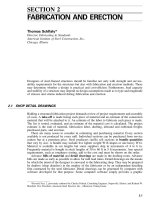
FIGURE 3.7 Forces acting on a truss. (a) Reactions R
L
and R
R
maintain equilibrium of the truss
under 20-kip load. (b) Forces acting on truss members cut by section A–A maintain equilibrium.

͚
F
ϭ
0 (3.11a)
x
͚
F
ϭ
0 (3.11b)
y
͚
M
ϭ
0 (3.11c)
where
͚
F
x
and
͚
F
y
are the sum of the components of the forces in the direction of the
perpendicular axes x and y, respectively, and
͚
M is the sum of the moments of all forces
about any point in the plane of the forces.
Figure 3.7a shows a truss that is in equilibrium under a 20-kip (20,000-lb) load. By Eq.
(3.11), the sum of the reactions, or forces R
L

and R
R
, needed to support the truss, is 20 kips.
(The process of determining these reactions is presented in Art. 3.29.) The sum of the
moments of all external forces about any point is zero. For instance, the moment of the
forces about the right support reaction R
R
is
͚
M
ϭ
(30
ϫ
20)
Ϫ
(40
ϫ
15)
ϭ
600
Ϫ
600
ϭ
0
(Since only vertical forces are involved, the equilibrium equation for horizontal forces does
not apply.)
A free-body diagram of a portion of the truss to the left of section AA is shown in Fig.
3.7b). The internal forces in the truss members cut by the section must balance the external
force and reaction on that part of the truss; i.e., all forces acting on the free body must
satisfy the three equations of equilibrium [Eq. (3.11)].

For three-dimensional structures, the equations of equilibrium may be written
͚
F
ϭ
0
͚
F
ϭ
0
͚
F
ϭ
0 (3.12a)
xyz
͚
M
ϭ
0
͚
M
ϭ
0
͚
M
ϭ
0 (3.12b)
xyz
The three force equations [Eqs. (3.12a)] state that for a body in equilibrium there is no
resultant force producing a translation in any of the three principal directions. The three
moment equations [Eqs. (3.12b)] state that for a body in equilibrium there is no resultant

moment producing rotation about any axes parallel to any of the three coordinate axes.
Furthermore, in statics, a structure is usually considered rigid or nondeformable, since
the forces acting on it cause very small deformations. It is assumed that no appreciable
changes in dimensions occur because of applied loading. For some structures, however, such
changes in dimensions may not be negligible. In these cases, the equations of equilibrium
should be defined according to the deformed geometry of the structure (Art. 3.46).
3.8
SECTION THREE
FIGURE 3.8 (a) Force F
AB
tends to slide body A along the surface of body B.(b)
Friction force F
ƒ
opposes motion.
(J. L. Meriam and L. G. Kraige, Mechanics, Part I: Statics, John Wiley & Sons, Inc.,
New York; F. P. Beer and E. R. Johnston, Vector Mechanics for Engineers—Statics and
Dynamics, McGraw-Hill, Inc., New York.)
3.5 FRICTIONAL FORCES
Suppose a body A transmits a force F
AB
onto a body B through a contact surface assumed
to be flat (Fig. 3.8a). For the system to be in equilibrium, body B must react by applying
an equal and opposite force F
BA
on body A. F
BA
may be resolved into a normal force N
and a force F
ƒ
parallel to the plane of contact (Fig. 3.8b). The direction of F

ƒ
is drawn to
resist motion.
The force F
ƒ
is called a frictional force. When there is no lubrication, the resistance to
sliding is referred to as dry friction. The primary cause of dry friction is the microscopic
roughness of the surfaces.
For a system including frictional forces to remain static (sliding not to occur), F
ƒ
cannot
exceed a limiting value that depends partly on the normal force transmitted across the surface
of contact. Because this limiting value also depends on the nature of the contact surfaces, it
must be determined experimentally. For example, the limiting value is increased considerably
if the contact surfaces are rough.
The limiting value of a frictional force for a body at rest is larger than the frictional force
when sliding is in progress. The frictional force between two bodies that are motionless is
called static friction, and the frictional force between two sliding surfaces is called sliding
or kinetic friction.
Experiments indicate that the limiting force for dry friction F
u
is proportional to the
normal force N:
F
ϭ
␮
N (3.13a)
us
where
␮

s
is the coefficient of static friction. For sliding not to occur, the frictional force F
ƒ
must be less than or equal to F
u
.IfF
ƒ
exceeds this value, sliding will occur. In this case,
the resulting frictional force is
F
ϭ
␮
N (3.13b)
kk
where
␮
k
is the coefficient of kinetic friction.
Consider a block of negligible weight resting on a horizontal plane and subjected to a
force P (Fig. 3.9a). From Eq. (3.1), the magnitudes of the components of P are
GENERAL STRUCTURAL THEORY
3.9
FIGURE 3.9 (a) Force P acting at an angle
␣
tends to slide block A against friction
with plane B.(b) When motion begins, the angle
␾
between the resultant R and the
normal force N is the angle of static friction.
P

ϭ
P sin
␣
(3.14a)
x
P
ϭ
P cos
␣
(3.14b)
y
For the block to be in equilibrium,
͚
F
x
ϭ
F
ƒ
Ϫ
P
x
ϭ
0 and
͚
F
y
ϭ
N
Ϫ
P

y
ϭ
0. Hence,
P
ϭ
F (3.15a)
x ƒ
P
ϭ
N (3.15b)
y
For sliding not to occur, the following inequality must be satisfied:
F
Յ
␮
N (3.16)
ƒ s
Substitution of Eqs. (3.15) into Eq. (3.16) yields
P
Յ
␮
P (3.17)
xsy
Substitution of Eqs. (3.14) into Eq. (3.17) gives
P sin
␣
Յ
␮
P cos
␣

s
which simplifies to
tan
␣
Յ
␮
(3.18)
s
This indicates that the block will just begin to slide if the angle
␣
is gradually increased to
the angle of static friction
␾
, where tan
␾
ϭ
␮
s
or
␾
ϭ
tan
Ϫ
1
␮
s
.
For the free-body diagram of the two-dimensional system shown in Fig. 3.9b, the resultant
force R
u

of forces F
u
and N defines the bounds of a plane sector with angle 2
␾
. For motion
not to occur, the resultant force R of forces F
ƒ
and N (Fig. 3.9a) must reside within this
plane sector. In three-dimensional systems, no motion occurs when R is located within a
cone of angle 2
␾
, called the cone of friction.
(F. P. Beer and E. R. Johnston, Vector Mechanics for Engineers—Statics and Dynamics,
McGraw-Hill, Inc., New York.)
3.10
SECTION THREE
STRUCTURAL MECHANICS—DYNAMICS
Dynamics is that branch of mechanics which deals with bodies in motion. Dynamics is
further divided into kinematics, the study of motion without regard to the forces causing
the motion, and kinetics, the study of the relationship between forces and resulting motions.
3.6 KINEMATICS
Kinematics relates displacement, velocity, acceleration, and time. Most engineering problems
in kinematics can be solved by assuming that the moving body is rigid and the motions
occur in one plane.
Plane motion of a rigid body may be divided into four categories: rectilinear translation,
in which all points of the rigid body move in straight lines; curvilinear translation, in
which all points of the body move on congruent curves; rotation, in which all particles
move in a circular path; and plane motion, a combination of translation and rotation in a
plane.
Rectilinear translation is often of particular interest to designers. Let an arbitrary point P

displace a distance
⌬
s to P
Ј
during time interval
⌬
t. The average velocity of the point during
this interval is
⌬
s/
⌬
t. The instantaneous velocity is obtained by letting
⌬
t approach zero:
⌬
sds
v ϭ
lim
ϭ
(3.19)
⌬
tdt
⌬
t
→
0
Let
⌬v
be the difference between the instantaneous velocities at points P and P
Ј

during the
time interval
⌬
t. The average acceleration is
⌬v
/
⌬
t. The instantaneous acceleration is
2
⌬v
d
v
ds
a
ϭ
lim
ϭϭ
(3.20)
2
⌬
tdtdt
⌬
t
→
0
Suppose, for example, that the motion of a particle is described by the time-dependent
displacement function s(t)
ϭ
t
4

Ϫ
2t
2
ϩ
1. By Eq. (3.19), the velocity of the particle would
be
ds
3
v ϭϭ
4t
Ϫ
4t
dt
By Eq. (3.20), the acceleration of the particle would be
2
d
v
ds
2
a
ϭϭ ϭ
12t
Ϫ
4
2
dt dt
With the same relationships, the displacement function s(t) could be determined from a
given acceleration function a(t). This can be done by integrating the acceleration function
twice with respect to time t. The first integration would yield the velocity function
v

(t)
ϭ
͐
a(t) dt, and the second would yield the displacement function s(t)
ϭ͐͐
a(t) dt dt.
These concepts can be extended to incorporate the relative motion of two points A and
B in a plane. In general, the displacement s
A
of A equals the vector sum of the displacement
of s
B
of B and the displacement s
AB
of A relative to B:
GENERAL STRUCTURAL THEORY
3.11
s
ϭ
s
ϩ
s (3.21)
ABAB
Differentiation of Eq. (3.21) with respect to time gives the velocity relation
v ϭ v ϩ v
(3.22)
ABAB
The acceleration of A is related to that of B by the vector sum
a
ϭ

a
ϩ
a (3.23)
ABAB
These equations hold for any two points in a plane. They need not be points on a rigid body.
(J. L. Meriam and L. G. Kraige, Mechanics, Part II: Dynamics, John Wiley & Son, Inc.,
New York; F. P. Beer and E. R. Johnston, Vector Mechanics for Engineers—Statics and
Dynamics, McGraw-Hill, Inc., New York.)
3.7 KINETICS
Kinetics is that part of dynamics that includes the relationship between forces and any
resulting motion.
Newton’s second law relates force and acceleration by
F
ϭ
ma (3.24)
where the force F and the acceleration a are vectors having the same direction, and the mass
m is a scalar.
The acceleration, for example, of a particle of mass m subject to the action of concurrent
forces, F
1
, F
2
, and F
3
, can be determined from Eq. (3.24) by resolving each of the forces
into three mutually perpendicular directions x, y, and z. The sums of the components in each
direction are given by
͚
F
ϭ

F
ϩ
F
ϩ
F (3.25a)
x 1x 2x 3x
͚
F
ϭ
F
ϩ
F
ϩ
F (3.25b)
y 1y 2y 3y
͚
F
ϭ
F
ϩ
F
ϩ
F (3.25c)
z 1z 2z 3z
The magnitude of the resultant of the three concurrent forces is
222
͚
F
ϭ ͙
(

͚
F )
ϩ
(
͚
F )
ϩ
(
͚
F ) (3.26)
xyz
The acceleration of the particle is related to the force resultant by
͚
F
ϭ
ma (3.27)
The acceleration can then be determined from
͚
F
a
ϭ
(3.28)
m
In a similar manner, the magnitudes of the components of the acceleration vector a are
3.12
SECTION THREE
2
dx
͚
F

x
a
ϭϭ
(3.29a)
x
2
dt m
2
dy
͚
F
y
a
ϭϭ
(3.29b)
y
2
dt m
2
dz
͚
F
z
a
ϭϭ
(3.29c)
z
2
dt m
Transformation of Eq. (3.27) into the form

͚
F
Ϫ
ma
ϭ
0 (3.30)
provides a condition in dynamics that often can be treated as an instantaneous condition in
statics; i.e., if a mass is suddenly accelerated in one direction by a force or a system of
forces, an inertia force ma will be developed in the opposite direction so that the mass
remains in a condition of dynamic equilibrium. This concept is known as d’Alembert’s
principle.
The principle of motion for a single particle can be extended to any number of particles
in a system:
͚
F
ϭ ͚
ma
ϭ
ma (3.31a)
xiixx
͚
F
ϭ ͚
ma
ϭ
ma (3.31b)
yiiyy
͚
F
ϭ ͚

ma
ϭ
ma (3.31c)
ziizz
where, for example,
͚
F
x
ϭ
algebraic sum of all x-component forces acting on the system
of particles
͚
m
i
a
ix
ϭ
algebraic sum of the products of the mass of each particle and
the x component of its acceleration
m
ϭ
total mass of the system
x
ϭ
a acceleration of the center of the mass of the particles in the x
direction
Extension of these relationships permits calculation of the location of the center of mass
(centroid for a homogeneous body) of an object:
͚
mx

ii
x
ϭ
(3.32a)
m
͚
my
ii
y
ϭ
(3.32b)
m
͚
mz
ii
z
ϭ
(3.32c)
m
where
ϭ
x, y, z coordinates of center of mass of the system
m
ϭ
total mass of the system
͚
m
i
x
i

ϭ
algebraic sum of the products of the mass of each particle and its x coor-
dinate
͚
m
i
y
i
ϭ
algebraic sum of the products of the mass of each particle and its y coor-
dinate
͚
m
i
z
i
ϭ
algebraic sum of the products of the mass of each particle and its z coor-
dinate
GENERAL STRUCTURAL THEORY
3.13
Concepts of impulse and momentum are useful in solving problems where forces are
expressed as a function of time. These problems include both the kinematics and the kinetics
parts of dynamics.
By Eqs. (3.29), the equations of motion of a particle with mass m are
d
v
x
͚
F

ϭ
ma
ϭ
m (3.33a)
xx
dt
d
v
y
͚
F
ϭ
ma
ϭ
m (3.33b)
yy
dt
d
v
z
͚
F
ϭ
ma
ϭ
m (3.33c)
zz
dt
Since m for a single particle is constant, these equations also can be written as
͚

Fdt
ϭ
d(m
v
) (3.34a)
xx
͚
Fdt
ϭ
d(m
v
) (3.34b)
yy
͚
Fdt
ϭ
d(m
v
) (3.34c)
zz
The product of mass and linear velocity is called linear momentum. The product of force
and time is called linear impulse.
Equations (3.34) are an alternate way of stating Newton’s second law. The action of
͚
F
x
,
͚
F
y

, and
͚
F
z
during a finite interval of time t can be found by integrating both sides of Eqs.
(3.34):
t
1
͵
͚
Fdt
ϭ
m(
v
)
Ϫ
m(
v
) (3.35a)
xxtxt
10
t
0
t
1
͵
͚
Fdt
ϭ
m(

v
)
Ϫ
m(
v
) (3.35b)
yytyt
10
t
0
t
1
͵
͚
Fdt
ϭ
m(
v
)
Ϫ
m(
v
) (3.35c)
zztzt
10
t
0
That is, the sum of the impulses on a body equals its change in momentum.
(J. L. Meriam and L. G. Kraige, Mechanics, Part II: Dynamics, John Wiley & Sons, Inc.,
New York; F. P. Beer and E. R. Johnston, Vector Mechanics for Engineers—Statics and

Dynamics, McGraw-Hill, Inc., New York.)
MECHANICS OF MATERIALS
Mechanics of materials, or strength of materials, incorporates the strength and stiffness
properties of a material into the static and dynamic behavior of a structure.
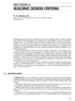
3.8 STRESS-STRAIN DIAGRAMS
Suppose that a homogeneous steel bar with a constant cross-sectional area A is subjected to
tension under axial load P (Fig. 3.10a). A gage length L is selected away from the ends of
3.14
SECTION THREE
FIGURE 3.10 Elongations of test specimen (a) are
measured from gage length L and plotted in (b) against
load.
the bar, to avoid disturbances by the end attachments that apply the load. The load P is
increased in increments, and the corresponding elongation
␦
of the original gage length is
measured. Figure 3.10b shows the plot of a typical load-deformation relationship resulting
from this type of test.
Assuming that the load is applied concentrically, the strain at any point along the gage
length will be
␧ ϭ
␦
/L, and the stress at any point in the cross section of the bar will be ƒ
ϭ
P/A. Under these conditions, it is convenient to plot the relation between stress and strain.
Figure 3.11 shows the resulting plot of a typical stress-stain relationship resulting from this
test.
3.9 COMPONENTS OF STRESS AND STRAIN
Suppose that a plane cut is made through a solid in equilibrium under the action of some
forces (Fig. 3.12a). The distribution of force on the area A in the plane may be represented

by an equivalent resultant force R
A
through point O (also in the plane) and a couple pro-
ducing moment M
A
(Fig. 3.12b).
Three mutually perpendicular axes x, y, and z at point O are chosen such that axis x is
normal to the plane and y and z are in the plane. R
A
can be resolved into components R
x
,
R
y
, and R
z
, and M
A
can be resolved into M
x
, M
y
, and M
z
(Fig. 3.12c). Component R
x
is
called normal force. R
y
and R

z
are called shearing forces. Over area A, these forces produce
an average normal stress R
x
/A and average shear stresses R
y
/A and R
z
/A, respectively. If
the area of interest is shrunk to an infinitesimally small area around point O, then the average
stresses would approach limits, called stress components, ƒ
x
,
v
xy
, and
v
xz
, at point O. Thus,
as indicated in Fig. 3.12d,
R
x
ƒ
ϭ
lim (3.36a)
ͩͪ
x
A
A
→

0
R
y
v ϭ
lim (3.36b)
ͩͪ
xy
A
A
→
0
R
z
v ϭ
lim (3.36c)
ͩͪ
xz
A
A
→
0
Because the moment M
A
and its corresponding components are all taken about point O, they
are not producing any additional stress at this point.
GENERAL STRUCTURAL THEORY
3.15
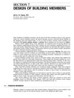
FIGURE 3.11 (a) Stress-strain diagram for A36 steel. (b) Portion of that diagram in the
yielding range.
If another plane is cut through O that is normal to the y axis, the area surrounding O in

this plane will be subjected to a different resultant force and moment through O. If the area
is made to approach zero, the stress components ƒ
y
,
v
yx
, and
v
yz
are obtained. Similarly, if a
third plane cut is made through O, normal to the z direction, the stress components are ƒ
z
,
v
zx
,
v
zy
.
The normal-stress component is denoted by ƒ and a single subscript, which indicates the
direction of the axis normal to the plane. The shear-stress component is denoted by
v
and
two subscripts. The first subscript indicates the direction of the normal to the plane, and the
second subscript indicates the direction of the axis to which the component is parallel.
The state of stress at a point O is shown in Fig. 3.13 on a rectangular parallelepiped with
length of sides
⌬
x,
⌬

y, and
⌬
x. The parallelepiped is taken so small that the stresses can be
3.16
SECTION THREE
FIGURE 3.12 Stresses at a point in a body due to external loads. (a) Forces acting on the
body. (b) Forces acting on a portion of the body. (c) Resolution of forces and moments about
coordinate axes through point O.(d) Stresses at point O.
FIGURE 3.13 Components of stress at a point.
considered uniform and equal on parallel faces. The stress at the point can be expressed by
the nine components shown. Some of these components, however, are related by equilibrium
conditions:
v ϭ vvϭ vvϭ v
(3.37)
xy yx yz zy zx xz
Therefore, the actual state of stress has only six independent components.
GENERAL STRUCTURAL THEORY
3.17
FIGURE 3.14 (a) Normal deformation. (b) Shear deformation.
A component of strain corresponds to each component of stress. Normal strains
␧
x
,
␧
y
,
and
␧
z
are the changes in unit length in the x, y, and z directions, respectively, when the

deformations are small (for example,
⑀
x
is shown in Fig. 3.14a). Shear strains
␥
xy
,
␥
zy
, and
␥
zx
are the decreases in the right angle between lines in the body at O parallel to the x and
y, z and y, and z and x axes, respectively (for example,
␥
xy
is shown in Fig. 3.14b). Thus,
similar to a state of stress, a state of strain has nine components, of which six are indepen-
dent.
3.10 STRESS-STRAIN RELATIONSHIPS
Structural steels display linearly elastic properties when the load does not exceed a certain
limit. Steels also are isotropic; i.e., the elastic properties are the same in all directions. The
material also may be assumed homogeneous, so the smallest element of a steel member
possesses the same physical property as the member. It is because of these properties that
there is a linear relationship between components of stress and strain. Established experi-
mentally (see Art. 3.8), this relationship is known as Hooke’s law. For example, in a bar
subjected to axial load, the normal strain in the axial direction is proportional to the normal
stress in that direction, or
ƒ
␧ ϭ

(3.38)
E
where E is the modulus of elasticity, or Young’s modulus.
If a steel bar is stretched, the width of the bar will be reduced to account for the increase
in length (Fig. 3.14a). Thus the normal strain in the x direction is accompanied by lateral
strains of opposite sign. If
⑀
x
is a tensile strain, for example, the lateral strains in the y and
z directions are contractions. These strains are related to the normal strain and, in turn, to
the normal stress by
ƒ
x
␧ ϭϪ
␯
␧ ϭϪ
␯
(3.39a)
yx
E
ƒ
x
␧ ϭϪ
␯
␧ ϭϪ
␯
(3.39b)
zx
E
where

␯
is a constant called Poisson’s ratio.
If an element is subjected to the action of simultaneous normal stresses ƒ
x
,ƒ
y
, and ƒ
z
uniformly distributed over its sides, the corresponding strains in the three directions are
3.18
SECTION THREE
1
␧ ϭ
[ƒ
Ϫ
␯
(ƒ
ϩ
ƒ )] (3.40a)
xxyz
E
1
␧ ϭ
[ƒ
Ϫ
␯
(ƒ
ϩ
ƒ )] (3.40b)
yyxz

E
1
␧ ϭ
[ƒ
Ϫ
␯
(ƒ
ϩ
ƒ )] (3.40c)
zzxy
E
Similarly, shear strain
␥
is linearly proportional to shear stress
v
vv
v
xy yz
zx
␥
ϭ
␥
ϭ
␥
ϭ
(3.41)
xy yz zx
GGG
where the constant G is the shear modulus of elasticity, or modulus of rigidity. For an
isotropic material such as steel, G is directly proportional to E:

E
G
ϭ
(3.42)
2(1
ϩ
␯
)
The analysis of many structures is simplified if the stresses are parallel to one plane. In
some cases, such as a thin plate subject to forces along its edges that are parallel to its plane
and uniformly distributed over its thickness, the stress distribution occurs all in one plane.
In this case of plane stress, one normal stress, say ƒ
z
, is zero, and corresponding shear
stresses are zero:
v
zx
ϭ
0 and
v
zy
ϭ
0.
In a similar manner, if all deformations or strains occur within a plane, this is a condition
of plane strain. For example,
␧
z
ϭ
0,
␥

zx
ϭ
0, and
␥
zy
ϭ
0.
3.11 PRINCIPAL STRESSES AND MAXIMUM SHEAR STRESS
When stress components relative to a defined set of axes are given at any point in a condition
of plane stress or plane strain (see Art. 3.10), this state of stress may be expressed with
respect to a different set of axes that lie in the same plane. For example, the state of stress
at point O in Fig. 3.15a may be expressed in terms of either the x and y axes with stress
components, ƒ
x
,ƒ
y
, and
v
xy
or the x
Ј
and y
Ј
axes with stress components , andƒ,ƒ
v
x
Ј
y
Ј
x

Ј
y
Ј
(Fig. 3.15b). If stress components ƒ
x
,ƒ
y
, and
v
xy
are given and the two orthogonal coordinate
systems differ by an angle
␣
with respect to the original x axis, the stress components ,ƒ
x
Ј
, and can be determined by statics. The transformation equations for stress areƒ
v
y
Ј
x
Ј
y
Ј
11
ƒ
ϭ
⁄
2
(ƒ

ϩ
ƒ)
ϩ
⁄
2
(ƒ
Ϫ
ƒ ) cos 2
␣
ϩ v
sin 2
␣
(3.43a)
x
Ј
xy xy xy
11
ƒ
ϭ
⁄
2
(ƒ
ϩ
ƒ)
Ϫ
⁄
2
(ƒ
Ϫ
ƒ ) cos 2

␣
Ϫ v
sin 2
␣
(3.43b)
y
Ј
xy xy xy
1
v ϭϪ
⁄
2
(ƒ
Ϫ
ƒ ) sin 2
␣
ϩ v
cos 2
␣
(3.43c)
x
Ј
y
Ј
xy xy
From these equations, an angle
␣
p
can be chosen to make the shear stress equal zero.
v

x
Ј
y
Ј
From Eq. (3.43c), with
ϭ
0,
v
x
Ј
y
Ј
2
v
xy
tan 2
␣
ϭ
(3.44)
p
ƒ
Ϫ
ƒ
xy
GENERAL STRUCTURAL THEORY
3.19
FIGURE 3.15 (a) Stresses at point O on planes perpendicular to x and y axes. (b) Stresses
relative to rotated axes.
This equation indicates that two perpendicular directions,
␣

p
and
␣
p
ϩ
(
␲
/2), may be found
for which the shear stress is zero. These are called principal directions. On the plane for
which the shear stress is zero, one of the normal stresses is the maximum stress ƒ
1
and the
other is the minimum stress ƒ
2
for all possible states of stress at that point. Hence the normal
stresses on the planes in these directions are called the principal stresses. The magnitude
of the principal stresses may be determined from
2
ƒ
ϩ
ƒƒ
Ϫ
ƒ
xy xy
2
ƒ
ϭ ע ϩ v
(3.45)
ͩͪ
xy

Ί
22
where the algebraically larger principal stress is given by ƒ
1
and the minimum principal
stress is given by ƒ
2
.
Suppose that the x and y directions are taken as the principal directions, that is,
v
xy
ϭ
0.
Then Eqs. (3.43) may be simplified to
11
ƒ
ϭ
⁄
2
(ƒ
ϩ
ƒ)
ϩ
⁄
2
(ƒ
Ϫ
ƒ ) cos 2
␣
(3.46a)

x
Ј
12 12
11
ƒ
ϭ
⁄
2
(ƒ
ϩ
ƒ)
Ϫ
⁄
2
(ƒ
Ϫ
ƒ ) cos 2
␣
(3.46b)
y
Ј
12 12
1
v ϭϪ
⁄
2
(ƒ
Ϫ
ƒ ) sin 2
␣

(3.46c)
x
Ј
y
Ј
12
By Eq. (3.46c), the maximum shear stress occurs when sin 2
␣
ϭ
␲
/2, i.e., when
␣
ϭ
45
Њ
. Hence the maximum shear stress occurs on each of two planes that bisect the angles
between the planes on which the principal stresses act. The magnitude of the maximum shear
stress equals one-half the algebraic difference of the principal stresses:
1
v ϭϪ
⁄
2
(ƒ
Ϫ
ƒ ) (3.47)
max 1 2
If on any two perpendicular planes through a point only shear stresses act, the state of
stress at this point is called pure shear. In this case, the principal directions bisect the angles
3.20
SECTION THREE

FIGURE 3.16 Mohr circle for obtaining, from principal stresses at a point, shear and
normal stresses on any plane through the point.
between the planes on which these shear stresses occur. The principal stresses are equal in
magnitude to the unit shear stress in each plane on which only shears act.
3.12 MOHR’S CIRCLE
Equations (3.46) for stresses at a point O can be represented conveniently by Mohr’s circle
(Fig. 3.16). Normal stress ƒ is taken as the abscissa, and shear stress
v
is taken as the ordinate.
The center of the circle is located on the ƒ axis at (ƒ
1
ϩ
ƒ
2
)/2, where ƒ
1
and ƒ
2
are the
maximum and minimum principal stresses at the point, respectively. The circle has a radius
of (ƒ
1
Ϫ
ƒ
2
)/2. For each plane passing through the point O there are two diametrically
opposite points on Mohr’s circle that correspond to the normal and shear stresses on the
plane. Thus Mohr’s circle can be used conveniently to find the normal and shear stresses on
a plane when the magnitude and direction of the principal stresses at a point are known.
Use of Mohr’s circle requires the principal stresses ƒ

1
and ƒ
2
to be marked off on the
abscissa (points A and B in Fig. 3.16, respectively). Tensile stresses are plotted to the right
of the
v
axis and compressive stresses to the left. (In Fig. 3.16, the principal stresses are
indicated as tensile stresses.) A circle is then constructed that has radius (ƒ
1
ϩ
ƒ
2
)/2 and
passes through A and B. The normal and shear stresses ƒ
x
,ƒ
y
, and
v
xy
on a plane at an angle
␣
with the principal directions are the coordinates of points C and D on the intersection of
GENERAL STRUCTURAL THEORY
3.21
the circle and the diameter making an angle 2
␣
with the abscissa. A counterclockwise angle
change

␣
in the stress plane represents a counterclockwise angle change of 2
␣
on Mohr’s
circle. The stresses ƒ
x
,
v
xy
, and ƒ
y
,
v
yx
on two perpendicular planes are represented on Mohr’s
circle by points (ƒ
x
,
Ϫ v
xy
) and (ƒ
y
,
v
yx
), respectively. Note that a shear stress is defined as
positive when it tends to produce counter-clockwise rotation of the element.
Mohr’s circle also can be used to obtain the principal stresses when the normal stresses
on two perpendicular planes and the shearing stresses are known. Figure 3.17 shows con-
struction of Mohr’s circle from these conditions. Points C (ƒ

x
,
v
xy
) and D (ƒ
y
,
Ϫ v
xy
) are
plotted and a circle is constructed with CD as a diameter. Based on this geometry, the
abscissas of points A and B that correspond to the principal stresses can be determined.
(I. S. Sokolnikoff, Mathematical Theory of Elasticity; S. P. Timoshenko and J. N. Goodier,
Theory of Elasticity; and Chi-Teh Wang, Applied Elasticity; and F. P. Beer and E. R. John-
ston, Mechanics of Materials, McGraw-Hill, Inc., New York; A. C. Ugural and S. K. Fenster,
Advanced Strength and Applied Elasticity, Elsevier Science Publishing, New York.)
BASIC BEHAVIOR OF STRUCTURAL COMPONENTS
The combination of the concepts for statics (Arts 3.2 to 3.5) with those of mechanics of
materials (Arts. 3.8 to 3.12) provides the essentials for predicting the basic behavior of
members in a structural system.
Structural members often behave in a complicated and uncertain way. To analyze the
behavior of these members, i.e., to determine the relationships between the external loads
and the resulting internal stresses and deformations, certain idealizations are necessary.
Through this approach, structural members are converted to such a form that an analysis of
their behavior in service becomes readily possible. These idealizations include mathematical
models that represent the type of structural members being assumed and the structural support
conditions (Fig. 3.18).
3.13 TYPES OF STRUCTURAL MEMBERS AND SUPPORTS
Structural members are usually classified according to the principal stresses induced by loads
that the members are intended to support. Axial-force members (ties or struts) are those

subjected to only tension or compression. A column is a member that may buckle under
compressive loads due to its slenderness. Torsion members, or shafts, are those subjected
to twisting moment, or torque. A beam supports loads that produce bending moments. A
beam-column is a member in which both bending moment and compression are present.
In practice, it may not be possible to erect truly axially loaded members. Even if it were
possible to apply the load at the centroid of a section, slight irregularities of the member
may introduce some bending. For analysis purposes, however, these bending moments may
often be ignored, and the member may be idealized as axially loaded.
There are three types of ideal supports (Fig. 3.19). In most practical situations, the support
conditions of structures may be described by one of these three. Figure 3.19a represents a
support at which horizontal movement and rotation are unrestricted, but vertical movement
is restrained. This type of support is usually shown by rollers. Figure 3.19b represents a
hinged, or pinned support, at which vertical and horizontal movements are prevented, while
only rotation is permitted. Figure 3.19c indicates a fixed support, at which no translation
or rotation is possible.
3.22
SECTION THREE
FIGURE 3.17 Mohr circle for determining principal stresses at a point.
3.14 AXIAL-FORCE MEMBERS
In an axial-force member, the stresses and strains are uniformly distributed over the cross
section. Typically examples of this type of member are shown in Fig. 3.20.
Since the stress is constant across the section, the equation of equilibrium may be written
as
P
ϭ
Aƒ (3.48)
where P
ϭ
axial load
ƒ

ϭ
tensile, compressive, or bearing stress
A
ϭ
cross-sectional area of the member
Similarly, if the strain is constant across the section, the strain
␧
corresponding to an axial
tensile or compressive load is given by
⌬
␧ ϭ
(3.49)
L
GENERAL STRUCTURAL THEORY
3.23
FIGURE 3.18 Idealization of (a) joist-and-girder framing by (b) concen-
trated loads on a simple beam.
FIGURE 3.19 Representation of types of ideal sup-
ports: (a) roller, (b) hinged support, (c) fixed support.
where L
ϭ
length of member
⌬ ϭ
change in length of member
Assuming that the material is an isotropic linear elastic medium (see Art. 3.9), Eqs. (3.48)
and (3.49) are related according to Hooke’s law
␧ ϭ
ƒ/E, where E is the modulus of elasticity
of the material. The change in length
⌬

of a member subjected to an axial load P can then
be expressed by
PL
⌬ ϭ
(3.50)
AE
Equation (3.50) relates the load applied at the ends of a member to the displacement of
one end of the member relative to the other end. The factor L/AE represents the flexibility
of the member. It gives the displacement due to a unit load.
Solving Eq. (3.50) for P yields
AE
P
ϭ ⌬
(3.51)
L
The factor AE/L represents the stiffness of the member in resisting axial loads. It gives the
magnitude of an axial load needed to produce a unit displacement.
Equations (3.50) to (3.51) hold for both tension and compression members. However,
since compression members may buckle prematurely, these equations may apply only if the
member is relatively short (Arts. 3.46 and 3.49).
3.24
SECTION THREE
FIGURE 3.20 Stresses in axially loaded members:
(a) bar in tension, (b) tensile stresses in bar, (c) strut
in compression, (d ) compressive stresses in strut.
FIGURE 3.21 (a) Circular shaft in torsion. (b) Deformation of a portion of the shaft. (c) Shear
in shaft.
3.15 MEMBERS SUBJECTED TO TORSION
Forces or moments that tend to twist a member are called torisonal loads. In shafts, the
stresses and corresponding strains induced by these loads depend on both the shape and size

of the cross section.
Suppose that a circular shaft is fixed at one end and a twisting couple, or torque, is
applied at the other end (Fig. 3.21a). When the angle of twist is small, the circular cross
section remains circular during twist. Also, the distance between any two sections remains
the same, indicating that there is no longitudinal stress along the length of the member.
Figure 3.21b shows a cylindrical section with length dx isolated from the shaft. The lower
cross section has rotated with respect to its top section through an angle d
␪
, where
␪
is the
GENERAL STRUCTURAL THEORY
3.25
total rotation of the shaft with respect to the fixed end. With no stress normal to the cross
section, the section is in a state of pure shear (Art. 3.9). The shear stresses act normal to
the radii of the section. The magnitude of the shear strain
␥
at a given radius r is given by
AA
Ј
d
␪
r
␪
22
␥
ϭϭ
r
ϭ
(3.52)

AA
Ј
dx L
1 2
where L
ϭ
total length of the shaft
d
␪
/dx
ϭ
␪
/L
ϭ
angle of twist per unit length of shaft
Incorporation of Hooke’s law (
v ϭ
G
␥
) into Eq. (3.52) gives the shear stress at a given
radius r:
Gr
␪
v ϭ
(3.53)
L
where G is the shear modulus of elasticity. This equation indicates that the shear stress in a
circular shaft varies directly with distance r from the axis of the shaft (Fig. 3.21c). The
maximum shear stress occurs at the surface of the shaft.
From conditions of equilibrium, the twisting moment T and the shear stress

v
are related
by
rT
v ϭ
(3.54)
J
where J
ϭ͐
r
2
dA
ϭ
␲
r
4
/2
ϭ
polar moment of inertia
dA
ϭ
differential area of the circular section
By Eqs. (3.53) and (3.54), the applied torque T is related to the relative rotation of one
end of the member to the other end by
GJ
T
ϭ
␪
(3.55)
L

The factor GJ/L represents the stiffness of the member in resisting twisting loads. It gives
the magnitude of a torque needed to produce a unit rotation.
Noncircular shafts behave differently under torsion from the way circular shafts do. In
noncircular shafts, cross sections do not remain plane, and radial lines through the centroid
do not remain straight. Hence the direction of the shear stress is not normal to the radius,
and the distribution of shear stress is not linear. If the end sections of the shaft are free to
warp, however, Eq. (3.55) may be applied generally when relating an applied torque T to
the corresponding member deformation
␪
. Table 3.1 lists values of J and maximum shear
stress for various types of sections.
(Torsional Analysis of Steel Members, American Institute of Steel Construction; F. Arbabi,
Structural Analysis and Behavior, McGraw-Hill, Inc., New York.)
3.16 BENDING STRESSES AND STRAINS IN BEAMS
Beams are structural members subjected to lateral forces that cause bending. There are dis-
tinct relationships between the load on a beam, the resulting internal forces and moments,
and the corresponding deformations.
Consider the uniformly loaded beam with a symmetrical cross section in Fig. 3.22. Sub-
jected to bending, the beam carries this load to the two supporting ends, one of which is
hinged and the other of which is on rollers. Experiments have shown that strains developed