Introduction to bayesian statistics
Bạn đang xem bản rút gọn của tài liệu. Xem và tải ngay bản đầy đủ của tài liệu tại đây (3.62 MB, 362 trang )
Preface
How This Text Was Developed
This text grew out of the course notes for an Introduction to Bayesian Statistics
course that I have been teaching at the University of Waikato for the past few years.
My goal in developing this course was to introduce Bayesian methods at the earliest
possible stage, and cover a similar range of topics as a traditional introductory
statistics course. There is currently an upsurge in using Bayesian methods in applied
statistical analysis, yet the Introduction to Statistics course most students take is
almost always taught from a frequentist perspective. In my view, this is not right.
Students with a reasonable mathematics background should be exposed to Bayesian
methods from the beginning, because that is the direction applied statistics is moving.
Mathematical Background Required
Bayesian statistics uses the rules of probability to make inferences, so students must
have good algebraic skills for recognizing and manipulating formulas. A general
knowledge of calculus would be an advantage in reading this book. In particular, the
student should understand that the area under a curve is found by integration, and
that the location of a maximum or a minimum of a continuous differentiable function
is found by setting the derivative function equal to zero and solving. The book is
self-contained with a calculus appendix students can refer to. However, the actual
calculus used is minimal.
xiii
xiv
PREFACE
Features of the Text
In this text I have introduced Bayesian methods using a step by step development from
conditional probability. In Chapter 4, the universe of an experiment is set up with
two dimensions, the horizontal dimension is observable, and the vertical dimension
is unobservable. Unconditional probabilities are found for each point in the universe
using the multiplication rule and the prior probabilities of the unobservable events.
Conditional probability is the probability on that part of the universe that occurred, the
reduced universe. It is found by dividing the unconditional probability by their sum
over all the possible unobservable events. Because of way the universe is organized,
this summing is down the column in the reduced universe. The division scales them
up so the conditional probabilities sum to one. This result known as Bayes’ theorem
is the key to this course. In Chapter 6 this pattern is repeated with the Bayesian
universe. The horizontal dimension is the sample space, the set of all possible values
of the observable random variable. The vertical dimension is the parameter space,
the set of all possible values of the unobservable parameter. The reduced universe
is the vertical slice that we observed. The conditional probabilities given what
we observed are the unconditional probabilities found by using the multiplication
rule (prior × likelihood) divided by their sum over all possible parameter values.
Again, this sum is taken down the column. The division rescales the probabilities
so they sum to one. This gives Bayes’ theorem for a discrete parameter and a
discrete observation. When the parameter is continuous, the rescaling is done by
dividing the joint probability-probability density function at the observed value by
its integral over all possible parameter values so it integrates to one. Again, the joint
probability-probability density function is found by the multiplication rule and at the
observed value is (prior × likelihood). This is done for binomial observations and a
continuous beta prior in Chapter 8. When the observation is also a continuous random
variable, the conditional probability density is found by rescaling the joint probability
density at the observed value by dividing by its integral over all possible parameter
values. Again, the joint probability density is found by the multiplication rule and at
the observed value is prior × likelihood. This is done for normal observations and
a continuous normal prior in Chapter 10. All these cases follow the same general
pattern.
Bayes’ theorem allows one to revise his/her belief about the parameter, given the
data that occurred. There must be a prior belief to start from. One’s prior distribution
gives the relative belief weights he/she has for the possible values of the parameters.
How to choose ones prior is discussed in detail. Conjugate priors are found by
matching first two moments with prior belief on location and spread. When the
conjugate shape does not give satisfactory representation of prior belief, setting up a
discrete prior and interpolating is suggested.
Details that I consider beyond the scope of this course are included as footnotes.
There are many figures that illustrate the main ideas, and there are many fully
worked out examples. I have included chapters comparing Bayesian methods with
the corresponding frequentist methods. There are exercises at the end of each chapter,
some with short answers. In the exercises, I only ask for the Bayesian methods to be
PREFACE
xv
used, because those are the methods I want the students to learn. There are computer
exercises to be done in Minitab or R using the included macros. Some of these
are small-scale Monte Carlo studies that demonstrate the efficiency of the Bayesian
methods evaluated according to frequentist criteria.
Advantages of the Bayesian Perspective
Anyone who has taught an Introduction to Statistics class will know that students have
a hard time coming to grips with statistical inference. The concepts of hypothesis
testing and confidence intervals are subtle and students struggle with them. Bayesian
statistics relies on a single tool, Bayes’ theorem to revise our belief given the data.
This is more like the kind of plausible reasoning that students use in their everyday
life, but structured in a formal way. Conceptually it is a more straightforward method
for making inferences. The Bayesian perspective offers a number of advantages over
the conventional frequentist perspective.
• The "objectivity" of frequentist statistics has been obtained by disregarding
any prior knowledge about the process being measured. Yet in science there
usually is some prior knowledge about the process being measured. Throwing
this prior information away is wasteful of information (which often translates
to money). Bayesian statistics uses both sources of information; the prior
information we have about the process and the information about the process
contained in the data. They are combined using Bayes’ theorem.
• The Bayesian approach allows direct probability statements about the parameters. This is much more useful to a scientist than the confidence statements
allowed by frequentist statistics. This is a very compelling reason for using
Bayesian statistics. Clients will interpret a frequentist confidence interval as a
probability interval. The statistician knows that that interpretation is not correct but also knows that the confidence interpretation relating the probability
to all possible data sets that could have occurred, but didn’t; is of no particular
use to the scientist. Why not use a perspective that allows them to make the
interpretation that is useful to them.
• Bayesian statistics has a single tool, Bayes’ theorem, which is used in all situations. This contrasts to frequentist procedures, which require many different
tools.
• Bayesian methods often outperform frequentist methods, even when judged by
frequentist criteria.
• Bayesian statistics has a straightforward way of dealing with nuisance parameters. They are always marginalized out of the joint posterior distribution.
• Bayes’ theorem gives the way to find the predictive distribution of future
observations. This is not always easily done in a frequentist way.
xvi
PREFACE
These advantages have been well known to statisticians for some time. However,
there were great difficulties in using Bayesian statistics in actual practice. While it is
easy to write down the formula for the posterior distribution,
g(θ|data) =
g(θ) × f (data|θ)
,
g(θ) × f (data|θ) dθ
a closed form existed only in a few simple cases, such as for a normal sample with
a normal prior. In other cases the integration required had to be done numerically.
This in itself made it more difficult for beginning students. If there were more than a
few parameters, it became extremely difficult to perform the numerical integration.
In the past few years, computer algorithms (e.g., the Gibbs Sampler and the
Metropolis-Hasting algorithm) have been developed to draw an (approximate) random sample from the posterior distribution, without having to completely evaluate
it. We can approximate the posterior distribution to any accuracy we wish by taking
a large enough random sample from it. This removes the disadvantage of Bayesian
statistics, for now it can be done in practice for problems with many parameters,
and for distributions from general samples and having general prior distributions.
Of course these methods are beyond the level of an introductory course. Nevertheless, we should be introducing our students the approach to statistics that gives the
theoretical advantages from the very start. That is how they will get the maximum
benefit.
Outline of a Course Based on This Text
At the University of Waikato we have a one-semester course based on this text. This
course consists of 36 one-hour lectures, 12 one-hour tutorial sessions, and several
computer assignments. In each tutorial session, the students work through a statistical
activity in a hands-on way. Some of the computer assignments involve Monte Carlo
studies showing the long run performance of statistical procedures.
• Chapter 1 (one lecture) gives an introduction to the course.
• Chapter 2 (three lectures) covers scientific data gathering including random
sampling methods and the need for randomized experiments to make inferences
on cause-effect relationships.
• Chapter 3 (two lectures) is on data analysis with methods for displaying and
summarizing data. If students have already covered this material in a previous
statistics course, this could be covered as a reading assignment only.
• Chapter 4 (three lectures) introduces the rules of probability including joint,
marginal, and conditional probability and shows Bayes’ theorem is the best
method for dealing with uncertainty.
• Chapter 5 (two lectures) introduces discrete and random variables.
PREFACE
xvii
• Chapter 6 ((three lectures) shows how Bayesian inference works for an discrete
random variable with a discrete prior.
• Chapter 7 (two lectures) introduces continuous random variables.
• Chapter 8 (three lectures) shows how inference is done on the population
proportion from a binomial sample using either a uniform or a beta prior.
There is discussion on choosing a beta prior that corresponds to your prior
belief, and graphing it to confirm that it fits your belief.
• Chapter 9 (three lectures) compares the Bayesian inferences for the proportion
with the corresponding frequentist ones. The Bayesian estimator for the proportion is compared with the corresponding frequentist estimator in terms of
mean squared error. The difference between the interpretations of Bayesian
credible interval and the frequentist confidence interval are discussed.
• Chapter 10 (four lectures) introduces Bayes’ theorem for the mean of a normal
distribution, using either a "flat" improper prior or a normal prior. There is
considerable discussion on choosing a normal prior, and graphing it to confirm
it fits with your belief. The predictive distribution of the next observation is
developed. Student’s t distribution is introduced as the adjustment required
for the credible intervals when the standard deviation is estimated from the
sample. Section 10.5 is at a higher level, and may be omitted.
• Chapter 11 (one lecture) compares the Bayesian inferences for mean with the
corresponding frequentist ones.
• Chapter 12 (three lectures) does Bayesian inference for the difference between
two normal means, and the difference between two binomial proportions using
the normal approximation.
• Chapter 13 (three lectures) does simple linear regression model in a Bayesian
manner. Section 13.5 is at a higher level, and may be omitted.
• Chapter 14 (three lectures) introduces robust Bayesian methods using mixture
priors. This chapter shows how to protect against misspecified priors, which
is one of the main concerns that many people have against using Bayesian
statistics. It is at a higher level than the previous chapters and could be omitted
and more lecture time given to the other chapters.
Acknowledgements
I would like to acknowledge the help I have had from many people. First, my
students over the past three years, whose enthusiasm with the early drafts encouraged
me to continue writing. My colleague, James Curran for writing the R macros,
and Appendix D on how to implement them, and giving me access to the glass
data. Ian Pool, Dharma Dharmalingam and Sandra Baxendine from the University of
xviii
PREFACE
Waikato Population Studies Centre for giving me access to the NZFEE data. Fiona
Petchey from the University of Waikato Carbon Dating Unit for giving me access to
the 14 C archeological data. Lance McKay from the University of Waikato Biology
Department for giving me access to the slug data. Graham McBride from NIWA
for giving me access to the New Zealand water quality data. Harold Henderson and
Neil Cox from AgResearch NZ for giving me access to the 13 C enriched Octanoic
acid breath test data, and the endophyte data. Martin Upsdell from AgResearch NZ
made some useful suggestions on an early draft. Renate Meyer from the University
of Auckland gave me useful comments on the manuscript. My colleagues Lyn Hunt,
Judi McWhirter, Murray Jorgensen, Ray Littler, Dave Whitaker and Nye John for
their support and encouragement through this project. Alec Zwart and Stephen Joe
for help with LATEX, and Karen Devoy for her secretarial assistance.
I would like to also thank my editor Rosalyn Farkas at John Wiley & Sons, and
Amy Hendrixson, of TeXnology Inc. for their patience and help through the process
from rough manuscript to camera-ready copy.
Finally, last but not least, I wish to thank my wife Sylvie for her constant love and
support and for her help on producing some of the figures.
WILLIAM M. "BILL" BOLSTAD
Hamilton, New Zealand
1
Introduction to
Statistical Science
Statistics is the science that relates data to specific questions of interest. This includes
devising methods to gather data relevant to the question, methods to summarize
and display the data to shed light on the question, and methods that enable us to
draw answers to the question that are supported by the data. Data almost always
contain uncertainty. This uncertainty may arise from selection of the items to be
measured, or it may arise from variability of the measurement process. Drawing
general conclusions from data is the basis for increasing knowledge about the world,
and is the basis for all rational scientific inquiry. Statistical inference gives us
methods and tools for doing this despite the uncertainty in the data. The methods
used for analysis depend on the way the data were gathered. It is vitally important
that there is a probability model explaining how the uncertainty gets into the data.
Showing a Causal Relationship from Data
Suppose we have observed two variables X and Y . Variable X appears to have an
association with variable Y . If high values of X occur with high values of variable Y
and low values of X occur with low values of Y , we say the association is positive. On
the other hand, the association could be negative in which high values of variable X
occur in with low values of variable Y . Figure 1.1 shows a schematic diagram where
the association is indicated by the dotted curve connecting X and Y . The unshaded
area indicates that X and Y are observed variables. The shaded area indicates that
there may be additional variables that have not been observed.
0 Introduction
to Bayesian Statistics. By William M. Bolstad
ISBN 0-471-27020-2 Copyright c John Wiley & Sons, Inc.
1
2
INTRODUCTION TO STATISTICAL SCIENCE
X
Y
Figure 1.1 Association between two variables.
X
Y
Figure 1.2 Association due to causal relationship.
We would like to determine why the two variables are associated. There are
several possible explanations. The association might be a causal one. For example,
X might be the cause of Y . This is shown in Figure 1.2, where the causal relationship
is indicated by the arrow from X to Y .
On the other hand, there could be an unidentified third variable Z that has a causal
effect on both X and Y . They are not related in a direct causal relationship. The
association between them is due to the effect of Z. Z is called a lurking variable,
since it is hiding in the background and it affects the data. This is shown in Figure
1.3.
It is possible that both a causal effect and a lurking variable may both be contributing to the association. This is shown in Figure 1.4. We say that the causal effect and
the effect of the lurking variable are confounded. This means that both effects are
included in the association.
THE SCIENTIFIC METHOD: A PROCESS FOR LEARNING
X
3
Y
Z
Figure 1.3 Association due to lurking variable.
X
Y
Z
Figure 1.4 Confounded causal and lurking variable effects.
Our first goal is to determine which of the possible reasons for the association
holds. If we conclude that it is due to a causal effect, then our next goal is to
determine the size of the effect. If we conclude that the association is due to causal
effect confounded with the effect of a lurking variable, then our next goal becomes
determining the sizes of both the effects.
1.1
THE SCIENTIFIC METHOD: A PROCESS FOR LEARNING
In the Middle Ages, science was deduced from principles set down many centuries
earlier by authorities such as Aristotle. The idea that scientific theories should be
tested against real world data revolutionized thinking. This way of thinking known
as the scientific method sparked the Renaissance.
The scientific method rests on the following premises:
• A scientific hypothesis can never be shown to be absolutely true.
4
INTRODUCTION TO STATISTICAL SCIENCE
• However, it must potentially be disprovable.
• It is a useful model until it is established that it is not true.
• Always go for the simplest hypothesis, unless it can be shown to be false.
This last principle, elaborated by William of Ockham in the 13th century, is now
known as "Ockham’s razor" and is firmly embedded in science. It keeps science from
developing fanciful overly elaborate theories. Thus the scientific method directs
us through an improving sequence of models, as previous ones get falsified. The
scientific method generally follows the following procedure:
1. Ask a question or pose a problem in terms of the current scientific hypothesis.
2. Gather all the relevant information that is currently available. This includes
the current knowledge about parameters of the model.
3. Design an investigation or experiment that addresses the question from step 1.
The predicted outcome of the experiment should be one thing if the current
hypothesis is true, and something else if the hypothesis is false.
4. Gather data from the experiment.
5. Draw conclusions given the experimental results. Revise the knowledge about
the parameters to take the current results into account.
The scientific method searches for cause and effect relationships between an experimental variable and an outcome variable. In other words, how changing the
experimental variable results in a change to the outcome variable. Scientific modelling develops mathematical models of these relationships. Both of them need to
isolate the experiment from outside factors that could affect the experimental results. All outside factors that can be identified as possibly affecting the results
must be controlled. It is no coincidence that the earliest successes for the method
were in physics and chemistry where the few outside factors could be identified
and controlled. Thus there were no lurking variables. All other relevant variables
could be identified, and physically controlled by being held constant. That way
they would not affect results of the experiment, and the effect of the experimental
variable on the outcome variable could be determined. In biology, medicine, engineering, technology, and the social sciences it isn’t that easy to identify the relevant
factors that must be controlled. In those fields a different way to control outside
factors, because they can’t be identified beforehand and physically controlled.
1.2
THE ROLE OF STATISTICS IN THE SCIENTIFIC METHOD
Statistical methods of inference can be used when there is random variability in the
data. The probability model for the data is justified by the design of the investigation or
MAIN APPROACHES TO STATISTICS
5
experiment. This can extend the scientific method into situations where the relevant
outside factors cannot even be identified. Since we cannot identify these outside
factors, we cannot control them directly. The lack of direct control means the outside
factors will be affecting the data. There is a danger that the wrong conclusions could
be drawn from the experiment due to these uncontrolled outside factors.
The important statistical idea of randomization has been developed to deal with
this possibility. The unidentified outside factors can be "averaged out" by randomly
assigning each unit to either treatment or control group. This contributes variability
to the data. Statistical conclusions always have some uncertainty or error due to
variability in the data. We can develop a probability model of the data variability
based on the randomization used. Randomization not only reduces this uncertainty
due to outside factors, it also allows us to measure the amount of uncertainty that
remains using the probability model. Randomization lets us control the outside
factors statistically, by averaging out their effects.
Underlying this is the idea of a statistical population, consisting of all possible
values of the observations that could be made. The data consists of observations
taken from a sample of the population. For valid inferences about the population
parameters from the sample statistics, the sample must be "representative" of the
population. Amazingly, choosing the sample randomly is the most effective way to
get representative samples!
1.3
MAIN APPROACHES TO STATISTICS
There are two main philosophical approaches to statistics. The first is often referred to
as the frequentist approach. Sometimes it is called the classical approach. Procedures
are developed by looking at how they perform over all possible random samples. The
probabilities don’t relate to the particular random sample that was obtained. In many
ways this indirect method places the "cart before the horse."
The alternative approach that we take in this book is the Bayesian approach. It
applies the laws of probability directly to the problem. This offers many fundamental
advantages over the more commonly used frequentist approach. We will show these
advantages over the course of the book.
Frequentist Approach to Statistics
Most introductory statistics books take the frequentist approach to statistics, which
is based on the following ideas:
• Parameters, the numerical characteristics of the population, are fixed but unknown constants.
• Probabilities are always interpreted as long run relative frequency.
• Statistical procedures are judged by how well they perform in the long run over
an infinite number of hypothetical repetitions of the experiment.
6
INTRODUCTION TO STATISTICAL SCIENCE
Probability statements are only allowed for random quantities. The unknown
parameters are fixed, not random, so probability statements cannot be made about
their value. Instead, a sample is drawn from the population, and a sample statistic
is calculated. The probability distribution of the statistic over all possible random
samples from the population is determined, and is known as the sampling distribution
of the statistic. The parameter of the population will also be a parameter of the
sampling distribution. The probability statement that can be made about the statistic
based on its sampling distribution is converted to a confidence statement about the
parameter. The confidence is based on the average behavior of the procedure under
all possible samples.
Bayesian Approach to Statistics
The Reverend Thomas Bayes first discovered the theorem that now bears his name.
It was written up in a paper An Essay Towards Solving a Problem in the Doctrine of
Chances. This paper was found after his death by his friend Richard Price, who had
it published posthumously in the Philosophical Transactions of the Royal Society in
1763. Bayes showed how inverse probability could be used to calculate probability
of antecedent events from the occurrence of the consequent event. His methods were
adopted by Laplace and other scientists in the 19th century, but had largely fallen
from favor by the early 20th century. By mid 20th century interest in Bayesian
methods was renewed by De Finetti, Jeffreys, Savage, and Lindley, among others.
They developed a complete method of statistical inference based on Bayes’ theorem.
This book introduces the Bayesian approach to statistics. The ideas that form the
basis of the this approach are:
• Since we are uncertain about the true value of the parameters we will consider
them a random variable.
• The rules of probability are used directly to make inferences about the parameters.
• Probability statements about parameters must be interpreted as "degree of
belief." The prior distribution must be subjective. Each person can have
his/her own prior, which contains the relative weights that person gives to every
possible parameter value. It measures how "plausible" the person considers
each parameter value to be before observing the data.
• We revise our beliefs about parameters after getting the data by using Bayes’
theorem. This gives our posterior distribution which gives the relative weights
we give to each parameter value after analyzing the data. The posterior distribution comes from two sources: the prior distribution and the observed
data.
This has a number of advantages over the conventional frequentist approach. Bayes’
theorem is the only consistent way to modify our beliefs about the parameters given
the data that actually occurred. This means that the inference is based on the
MAIN APPROACHES TO STATISTICS
7
actual occurring data, not all possible data sets that might have occurred, but didn’t!
Allowing the parameter to be a random variable lets us make probability statements
about it, posterior to the data. This contrasts with the conventional approach where
inference probabilities are based on all possible data sets that could have occurred
for the fixed parameter value. Given the actual data there is nothing random left
with a fixed parameter value, so one can only make confidence statements, based
on what could have occurred. Bayesian statistics also has a general way of dealing
with a nuisance parameter . A nuisance parameter is one which we don’t want to
make inference about, but we don’t want them to interfere with the inferences we
are making about the main parameters. Frequentist statistics does not have a general
procedure for dealing with them. Bayesian statistics is predictive, unlike conventional
frequentist statistics. This means that we can easily find the conditional probability
distribution of the next observation given the sample data.
Monte Carlo Studies
In frequentist statistics, the parameter is considered a fixed, but unknown constant. A
statistical procedure such as a particular estimator for the parameter cannot be judged
from the value it takes given the data. The parameter is unknown, so we can’t know
the value it should be giving. If we knew the parameter value it was supposed to take,
we wouldn’t be using an estimator.
Instead, statistical procedures are evaluated by looking how they perform in the
long run over all possible samples of data, for fixed parameter values over some
range. For instance, we fix the parameter at some value. The estimator depends
on the random sample, so it is considered a random variable having a probability
distribution. This distribution is called the sampling distribution of the estimator,
since its probability distribution comes from taking all possible random samples.
Then we look at how the estimator is distributed around the parameter value. This is
called sample space averaging. Essentially it compares the performance of procedures
before we take any data.
Bayesian procedures consider the parameter to be a random variable, and its
posterior distribution is conditional on the sample data that actually occurred, not all
those samples that were possible, but did not occur. However, before the experiment,
we might want to know how well the Bayesian procedure works at some specific
parameter values in the range.
To evaluate the Bayesian procedure using sample space averaging, we have to
consider the parameter to be both a random variable and a fixed but unknown value
at the same time. We can get past the apparent contradiction in the nature of the
parameter because the probability distribution we put on the parameter measures
our uncertainty about the true value. It shows the relative belief weights we give to
the possible values of the unknown parameter! After looking at the data, our belief
distribution over the parameter values has changed. This way we can think of the
parameter as fixed, but unknown value at the same time as we think of it being a
random variable. This allows us to evaluate the Bayesian procedure using sample
8
INTRODUCTION TO STATISTICAL SCIENCE
space averaging. This is called pre-posterior analysis because it can be done before
we obtain the data.
In Chapter 4, we will find out that the laws of probability are the best way to model
uncertainty. Because of this, Bayesian procedures will be optimal in the post-data
setting, given the data that actually occurred. In Chapters 9 and 11, we will see
that Bayesian procedures perform very well in the pre-data setting when evaluated
using pre-posterior analysis. In fact, it is often the case that Bayesian procedures
outperform the usual frequentist procedures even in the pre-data setting.
Monte Carlo studies are a useful way to perform sample space averaging. We draw
a large number of samples randomly using the computer and calculate the statistic
(frequentist or Bayesian) for each sample. The empirical distribution of the statistic
(over the large number of random samples) approximates its sampling distribution
(over all possible random samples). We can calculate statistics such as mean and
standard deviation on this Monte Carlo sample to approximate the mean and standard
deviation of the sampling distribution. Some small-scale Monte Carlo studies are
included as exercises.
1.4
PURPOSE AND ORGANIZATION OF THIS TEXT
A very large proportion of undergraduates are required to take a service course in
statistics. Almost all of these courses are based on frequentist ideas. Most of them
don’t even mention Bayesian ideas. As a statistician, I know that Bayesian methods
have great theoretical advantages. I think we should be introducing our best students
to Bayesian ideas, from the beginning. There aren’t many introductory statistics text
books based on the Bayesian ideas. Some other texts include Berry (1996), Press
(1989), and Lee (1989).
This book aims to introduce students with a good mathematics background to
Bayesian statistics. It covers the same topics as a standard introductory statistics
text, only from a Bayesian perspective. Students need reasonable algebra skills to
follow this book. Bayesian statistics uses the rules of probability, so competence
in manipulating mathematical formulas is required. Students will find that general
knowledge of calculus is helpful in reading this book. Specifically they need to know
that area under a curve is found by integrating, and that a maximum or minimum
of a continuous differentiable function is found where the derivative of the function
equals zero. However the actual calculus used is minimal. The book is self-contained
with a calculus appendix students can refer to.
Chapter 2 introduces some fundamental principles of scientific data gathering
to control the effects of unidentified factors. These include the need for drawing
samples randomly, and some of random sampling techniques. The reason why there
is a difference between the conclusions we can draw from data arising from an
observational study and from data arising from a randomized experiment is shown.
Completely randomized designs and randomized block designs are discussed.
PURPOSE AND ORGANIZATION OF THIS TEXT
9
Chapter 3 covers elementary methods for graphically displaying and summarizing
data. Often a good data display is all that is necessary. The principles of designing
displays that are true to the data are emphasized.
Chapter 4 shows the difference between deduction and induction. Plausible reasoning is shown to be an extension of logic where there is uncertainty. It turns out that
plausible reasoning must follow the same rules as probability. The axioms of probability are introduced and the rules of probability, including conditional probability
and Bayes’ theorem are developed.
Chapter 5 covers discrete random variables, including joint and marginal discrete
random variables. The binomial and hypergeometric distributions are introduced,
and the situations where they arise are characterized.
Chapter 6 covers Bayes’ theorem for discrete random variables using a table. We
see that two important consequences of the method are that multiplying the prior by
a constant, or that multiplying the likelihood by a constant do not affect the resulting
posterior distribution. This gives us the "proportional form" of Bayes’ theorem.
We show that we get the same results when we analyze the observations sequentially
using the posterior after the previous observation as the prior for the next observation,
as when we analyze the observations all at once using the joint likelihood and the
original prior. We show how to use Bayes’ theorem for binomial observations with
a discrete prior.
Chapter 7 covers continuous random variables, including joint, marginal, and
conditional random variables. The beta and normal distributions are introduced in
this chapter.
Chapter 8 covers Bayes’ theorem for the population proportion (binomial) with a
continuous prior. We show how to find the posterior distribution of the population
proportion using either a uniform prior or a beta prior. We explain how to choose a
suitable prior. We look at ways of summarizing the posterior distribution.
Chapter 9 compares the Bayesian inferences with the frequentist inferences. We
show that the Bayesian estimator (posterior mean using a uniform prior) has better
performance than the frequentist estimator (sample proportion) in terms of mean
squared error over most of the range of possible values. This kind of frequentist
analysis is useful before we perform our Bayesian analysis. We see the Bayesian
credible interval has a much more useful interpretation than the frequentist confidence
interval for the population proportion. One-sided and two-sided hypothesis tests using
Bayesian methods are introduced.
Chapter 10 covers Bayes’ theorem for the mean of a normal distribution with
known variance. We show how to choose a normal prior. We discuss dealing
with nuisance parameters by marginalization. The predictive density of the next
observation is found by considering the population mean a nuisance parameter, and
marginalizing it out.
Chapter 11 compares Bayesian inferences with the frequentist inferences for the
mean of a normal distribution.
Chapter 12 shows how to perform Bayesian inferences for the difference between
normal means and how to perform Bayesian inferences for the difference between
proportions using the normal approximation.