Solution manual heat and mass transfer a practical approach 2nd edition cengel ch 6

Chapter 6 Fundamentals of Convection

Chapter 6
FUNDAMENTALS OF CONVECTION
Physical Mechanisms of Forced Convection
6-1C In forced convection, the fluid is forced to flow over a surface or in a tube by external means such as
a pump or a fan. In natural convection, any fluid motion is caused by natural means such as the buoyancy
effect that manifests itself as the rise of the warmer fluid and the fall of the cooler fluid. The convection
caused by winds is natural convection for the earth, but it is forced convection for bodies subjected to the
winds since for the body it makes no difference whether the air motion is caused by a fan or by the winds.
6-2C If the fluid is forced to flow over a surface, it is called external forced convection. If it is forced to
flow in a tube, it is called internal forced convection. A heat transfer system can involve both internal and
external convection simultaneously. Example: A pipe transporting a fluid in a windy area.
6-3C The convection heat transfer coefficient will usually be higher in forced convection since heat
transfer coefficient depends on the fluid velocity, and forced convection involves higher fluid velocities.
6-4C The potato will normally cool faster by blowing warm air to it despite the smaller temperature
difference in this case since the fluid motion caused by blowing enhances the heat transfer coefficient
considerably.
6-5C Nusselt number is the dimensionless convection heat transfer coefficient, and it represents the
enhancement of heat transfer through a fluid layer as a result of convection relative to conduction across
hL
where L is the characteristic length of the surface and k is
the same fluid layer. It is defined as Nu =
k
the thermal conductivity of the fluid.
6-6C Heat transfer through a fluid is conduction in the absence of bulk fluid motion, and convection in the
presence of it. The rate of heat transfer is higher in convection because of fluid motion. The value of the
convection heat transfer coefficient depends on the fluid motion as well as the fluid properties. Thermal
conductivity is a fluid property, and its value does not depend on the flow.
6-7C A fluid flow during which the density of the fluid remains nearly constant is called incompressible
flow. A fluid whose density is practically independent of pressure (such as a liquid) is called an

incompressible fluid. The flow of compressible fluid (such as air) is not necessarily compressible since the
density of a compressible fluid may still remain constant during flow.

6-1


Chapter 6 Fundamentals of Convection
6-8 Heat transfer coefficients at different air velocities are given during air cooling of potatoes. The initial
rate of heat transfer from a potato and the temperature gradient at the potato surface are to be determined.
Assumptions 1 Steady operating conditions exist. 2 Potato is spherical in shape. 3 Convection heat transfer
coefficient is constant over the entire surface.
Properties The thermal conductivity of the potato is given to be k = 0.49 W/m.°C.
Analysis The initial rate of heat transfer from a potato is

As = πD 2 = π (0.10 m) 2 = 0.03142 m 2

Air
V∞ = 1 m/s
T∞ = 5°C

Q& = hAs (Ts − T∞ ) = (19.1 W/m .°C)(0.03142 m )(20 − 5)°C = 9.0 W
2

2

where the heat transfer coefficient is obtained from the table at 1 m/s
velocity. The initial value of the temperature gradient at the potato
surface is

Potato

Ti = 20°C

⎛ ∂T ⎞
q& conv = q& cond = − k ⎜
= h(Ts − T∞ )
⎟
⎝ ∂r ⎠ r = R
∂T
∂r

=−
r =R

h(Ts − T∞ )
(19.1 W/m 2 .°C)(20 − 5)°C
=−
= −585 °C/m
k
(0.49 W/m.°C)

6-9 The rate of heat loss from an average man walking in still air is to be determined at different walking
velocities.
Assumptions 1 Steady operating conditions exist. 2 Convection heat transfer coefficient is constant over
the entire surface.
Analysis The convection heat transfer coefficients and the rate of heat losses at different walking velocities
are
(a) h = 8.6V 0.53 = 8.6(0.5 m/s) 0.53 = 5.956 W/m 2 .°C

Q& = hAs (Ts − T∞ ) = (5.956 W/m 2 .°C)(1.8 m 2 )(30 − 10)°C = 214.4 W
(b) h = 8.6V 0.53 = 8.6(1.0 m/s) 0.53 = 8.60 W/m 2 .°C

Q& = hAs (Ts − T∞ ) = (8.60 W/m 2 .°C)(1.8 m 2 )(30 − 10)°C = 309.6 W
(c) h = 8.6V 0.53 = 8.6(1.5 m/s) 0.53 = 10.66 W/m 2 .°C

Q& = hAs (Ts − T∞ ) = (10.66 W/m 2 .°C)(1.8 m 2 )(30 − 10)°C = 383.8 W
(d) h = 8.6V 0.53 = 8.6(2.0 m/s) 0.53 = 12.42 W/m 2 .°C

Q& = hAs (Ts − T∞ ) = (12.42 W/m 2 .°C)(1.8 m 2 )(30 − 10)°C = 447.0 W

6-2

Air
V∞
T∞ = 10°C

Ts = 30°C


Chapter 6 Fundamentals of Convection
6-10 The rate of heat loss from an average man walking in windy air is to be determined at different wind
velocities.
Assumptions 1 Steady operating conditions exist. 2 Convection heat transfer coefficient is constant over
the entire surface.
Analysis The convection heat transfer coefficients and the rate of heat losses at different wind velocities
are
(a) h = 14.8V 0.53 = 14.8(0.5 m/s) 0.69 = 9.174 W/m 2 .°C

Q& = hAs (Ts − T∞ ) = (9.174 W/m 2 .°C)(1.7 m 2 )(29 − 10)°C = 296.3 W

Ts = 29°C

Air
V∞
T∞ = 10°C

(b) h = 14.8V 0.53 = 14.8(1.0 m/s) 0.69 = 14.8 W/m 2 .°C

Q& = hAs (Ts − T∞ ) = (14.8 W/m 2 .°C)(1.7 m 2 )(29 − 10)°C = 478.0 W
(c) h = 14.8V 0.53 = 14.8(1.5 m/s) 0.69 = 19.58 W/m 2 .°C

Q& = hAs (Ts − T∞ ) = (19.58 W/m 2 .°C)(1.7 m 2 )(29 − 10)°C = 632.4 W
6-11 The expression for the heat transfer coefficient for air cooling of some fruits is given. The initial rate
of heat transfer from an orange, the temperature gradient at the orange surface, and the value of the Nusselt
number are to be determined.
Assumptions 1 Steady operating conditions exist. 2 Orange is spherical in shape. 3 Convection heat
transfer coefficient is constant over the entire surface. 4 Properties of water is used for orange.
Properties The thermal conductivity of the orange is given to be k = 0.50 W/m.°C. The thermal
conductivity and the kinematic viscosity of air at the film temperature of (Ts + T∞)/2 = (15+5)/2 = 10°C are
(Table A-15)
k = 0.02439 W/m.°C,
υ = 1.426 × 10 -5 m 2 /s
Analysis (a) The Reynolds number, the heat transfer coefficient, and the initial rate of heat transfer from an
orange are

As = πD 2 = π (0.07 m) 2 = 0.01539 m 2

Air
V∞=0.5 m/s
T∞ = 5°C

V D (0.5 m/s)(0.07 m)
Re = ∞ =
= 2454
υ
1.426 ×10 −5 m 2 /s
5.05k air Re1 / 3 5.05(0.02439 W/m.°C)(2454)1 / 3
h=
=
= 23.73 W/m 2 .°C
D
0.07 m

Q& = hAs (Ts − T∞ ) = (23.73 W/m 2 .°C)(0.01539 m 2 )(15 − 5)°C = 3.65 W
(b) The temperature gradient at the orange surface is determined from
⎛ ∂T ⎞
= h(Ts − T∞ )
q& conv = q& cond = − k ⎜
⎟
⎝ ∂r ⎠ r = R
∂T
∂r

=−
r =R

h(Ts − T∞ )
(23.73 W/m 2 .°C)(15 − 5)°C
=−
= −475 °C/m
k

(0.50 W/m.°C)

(c) The Nusselt number is Re =

hD (23.73 W/m 2 .°C)(0.07 m)
=
= 68.11
0.02439 W/m.°C
k

6-3

Orange
Ti = 15°C


Chapter 6 Fundamentals of Convection
Velocity and Thermal Boundary Layers
6-12C Viscosity is a measure of the “stickiness” or “resistance to deformation” of a fluid. It is due to the
internal frictional force that develops between different layers of fluids as they are forced to move relative
to each other. Viscosity is caused by the cohesive forces between the molecules in liquids, and by the
molecular collisions in gases. Liquids have higher dynamic viscosities than gases.
6-13C The fluids whose shear stress is proportional to the velocity gradient are called Newtonian fluids.
Most common fluids such as water, air, gasoline, and oils are Newtonian fluids.
6-14C A fluid in direct contact with a solid surface sticks to the surface and there is no slip. This is known
as the no-slip condition, and it is due to the viscosity of the fluid.
6-15C For the same cruising speed, the submarine will consume much less power in air than it does in
water because of the much lower viscosity of air relative to water.
6-16C (a) The dynamic viscosity of liquids decreases with temperature. (b) The dynamic viscosity of gases
increases with temperature.

6-17C The fluid viscosity is responsible for the development of the velocity boundary layer. For the
idealized inviscid fluids (fluids with zero viscosity), there will be no velocity boundary layer.
6-18C The Prandtl number Pr = ν / α is a measure of the relative magnitudes of the diffusivity of
momentum (and thus the development of the velocity boundary layer) and the diffusivity of heat (and thus
the development of the thermal boundary layer). The Pr is a fluid property, and thus its value is
independent of the type of flow and flow geometry. The Pr changes with temperature, but not pressure.
6-19C A thermal boundary layer will not develop in flow over a surface if both the fluid and the surface
are at the same temperature since there will be no heat transfer in that case.
Laminar and Turbulent Flows
6-20C A fluid motion is laminar when it involves smooth streamlines and highly ordered motion of
molecules, and turbulent when it involves velocity fluctuations and highly disordered motion. The heat
transfer coefficient is higher in turbulent flow.
6-21C Reynolds number is the ratio of the inertial forces to viscous forces, and it serves as a criteria for
determining the flow regime. For flow over a plate of length L it is defined as Re = VL/υ where V is flow
velocity and υ is the kinematic viscosity of the fluid.
6-22C The friction coefficient represents the resistance to fluid flow over a flat plate. It is proportional to
the drag force acting on the plate. The drag coefficient for a flat surface is equivalent to the mean friction
coefficient.
6-23C In turbulent flow, it is the turbulent eddies due to enhanced mixing that cause the friction factor to
be larger.
6-24C Turbulent viscosity μt is caused by turbulent eddies, and it accounts for momentum transport by
turbulent eddies. It is expressed as τ t = − ρ u ′v ′ = μ t

∂u
where u is the mean value of velocity in the
∂y

flow direction and u ′ and u ′ are the fluctuating components of velocity.

6-4

Chapter 6 Fundamentals of Convection
6-25C Turbulent thermal conductivity kt is caused by turbulent eddies, and it accounts for thermal energy
transport by turbulent eddies. It is expressed as

q& t = ρC p v ′T ′ = − k t

∂T
where T ′ is the eddy
∂y

temperature relative to the mean value, and q& t = ρC p v ′T ′ the rate of thermal energy transport by turbulent
eddies.
Convection Equations and Similarity Solutions
6-26C A curved surface can be treated as a flat surface if there is no flow separation and the curvature
effects are negligible.
6-27C The continuity equation for steady two-dimensional flow is expressed as

∂u ∂v
+
= 0 . When
∂x ∂y

multiplied by density, the first and the second terms represent net mass fluxes in the x and y directions,
respectively.
6-28C Steady simply means no change with time at a specified location (and thus ∂u / ∂t = 0 ), but the
value of a quantity may change from one location to another (and thus ∂u / ∂x and ∂u / ∂y may be
different from zero). Even in steady flow and thus constant mass flow rate, a fluid may accelerate. In the
case of a water nozzle, for example, the velocity of water remains constant at a specified point, but it

changes from inlet to the exit (water accelerates along the nozzle).
6-29C In a boundary layer during steady two-dimensional flow, the velocity component in the flow
direction is much larger than that in the normal direction, and thus u >> v, and ∂v / ∂x and ∂v / ∂y are
negligible. Also, u varies greatly with y in the normal direction from zero at the wall surface to nearly the
free-stream value across the relatively thin boundary layer, while the variation of u with x along the flow is
typically small. Therefore, ∂u / ∂y >> ∂u / ∂x . Similarly, if the fluid and the wall are at different
temperatures and the fluid is heated or cooled during flow, heat conduction will occur primarily in the
direction normal to the surface, and thus ∂T / ∂y >> ∂T / ∂x . That is, the velocity and temperature
gradients normal to the surface are much greater than those along the surface. These simplifications are
known as the boundary layer approximations.
6-30C For flows with low velocity and for fluids with low viscosity the viscous dissipation term in the
energy equation is likely to be negligible.
6-31C For steady two-dimensional flow over an isothermal flat plate in the x-direction, the boundary
conditions for the velocity components u and v, and the temperature T at the plate surface and at the edge
of the boundary layer are expressed as follows:
T∞
u∞, T∞
At y = 0:
u(x, 0) = 0,
v(x, 0) = 0, T(x, 0) = Ts
y
As y → ∞ :
u(x, ∞) = u∞, T(x, ∞) = T∞
6-32C An independent variable that makes it possible to transforming a setx of partial differential equations
into a single ordinary differential equation is called a similarity variable. A similarity solution is likely to
exist for a set of partial differential equations if there is a function that remains unchanged (such as the
non-dimensional velocity profile on a flat plate).
6-33C During steady, laminar, two-dimensional flow over an isothermal plate, the thickness of the
velocity boundary layer (a) increase with distance from the leading edge, (b) decrease with free-stream
velocity, and (c) and increase with kinematic viscosity

6-34C During steady, laminar, two-dimensional flow over an isothermal plate, the wall shear stress
decreases with distance from the leading edge

6-5


Chapter 6 Fundamentals of Convection

6-35C A major advantage of nondimensionalizing the convection equations is the significant reduction in
the number of parameters [the original problem involves 6 parameters (L, V , T∞, Ts, ν, α), but the
nondimensionalized problem involves just 2 parameters (ReL and Pr)]. Nondimensionalization also results
in similarity parameters (such as Reynolds and Prandtl numbers) that enable us to group the results of a
large number of experiments and to report them conveniently in terms of such parameters.
6-36C For steady, laminar, two-dimensional, incompressible flow with constant properties and a Prandtl
number of unity and a given geometry, yes, it is correct to say that both the average friction and heat
transfer coefficients depend on the Reynolds number only since C f = f 4 (Re L ) and Nu = g 3 (Re L , Pr)
from non-dimensionalized momentum and energy equations.

6-6


Chapter 6 Fundamentals of Convection
6-37 Parallel flow of oil between two plates is considered. The velocity and temperature distributions, the
maximum temperature, and the heat flux are to be determined.
Assumptions 1 Steady operating conditions exist. 2 Oil is an incompressible substance with constant
properties. 3 Body forces such as gravity are negligible. 4 The plates are large so that there is no variation
in z direction.
Properties The properties of oil at the average temperature of (40+15)/2 = 27.5°C are (Table A-13):
k = 0.145 W/m-K

and

μ = 0.580 kg/m-s = 0.580 N-s/m2

Analysis (a) We take the x-axis to be the flow direction, and y to be the normal direction. This is parallel
flow between two plates, and thus v = 0. Then the continuity equation reduces to
∂u ∂v
∂u
+
= 0 ⎯→
⎯→ u = u(y)
Continuity:
=0
∂x
∂x ∂y
12 m/s
Therefore, the x-component of velocity does not change in the
flow direction (i.e., the velocity profile remains unchanged).
T2=40°C
Noting that u = u(y), v = 0, and ∂P / ∂x = 0 (flow is maintained
by the motion of the upper plate rather than the pressure
L=0.7 mm
Oil
gradient), the x-momentum equation (Eq. 6-28) reduces to
⎛ ∂u
d 2u
∂u ⎞
∂ 2 u ∂P
⎯→ 2 = 0
+ v ⎟⎟ = μ 2 −

ρ⎜⎜ u
x-momentum:
T1=25°C
∂y ⎠
∂x
dy
∂y
⎝ ∂x
This is a second-order ordinary differential equation, and integrating it twice gives
u ( y ) = C1 y + C 2

The fluid velocities at the plate surfaces must be equal to the velocities of the plates because of the no-slip
condition. Therefore, the boundary conditions are u(0) = 0 and u(L) = V , and applying them gives the
velocity distribution to be
u( y) =

y
V
L

Frictional heating due to viscous dissipation in this case is significant because of the high
viscosity of oil and the large plate velocity. The plates are isothermal and there is no change in the flow
direction, and thus the temperature depends on y only, T = T(y). Also, u = u(y) and v = 0. Then the energy
equation with dissipation (Eqs. 6-36 and 6-37) reduce to
2

⎛ ∂u ⎞
d 2T
⎛V⎞
⎜⎜ ⎟⎟

+
μ
⎯→
k
= −μ ⎜ ⎟
2
∂
y
∂y 2
dy
⎝L⎠
⎝ ⎠
since ∂u / ∂y = V / L . Dividing both sides by k and integrating twice give
Energy:

0=k

∂ 2T

2

2

T ( y) = −

μ ⎛y ⎞
⎜ V⎟ + C3 y + C 4
2k ⎝ L ⎠

Applying the boundary conditions T(0) = T1 and T(L) = T2 gives the temperature distribution to be

T ( y) =

T2 − T1
μV 2
y + T1 +
L
2k

⎛ y y2 ⎞
⎜ −
⎟
⎜ L L2 ⎟
⎝
⎠

(b) The temperature gradient is determined by differentiating T(y) with respect to y,

y⎞
dT T2 − T1 μV 2 ⎛
=
+
⎜1 − 2 ⎟
dy
L
2kL ⎝
L⎠
The location of maximum temperature is determined by setting dT/dy = 0 and solving for y,
⎛ T −T 1 ⎞
y⎞
dT T2 − T1 μV 2 ⎛

y = L⎜ k 2 2 1 + ⎟
=
+
⎯→
⎜1 − 2 ⎟ = 0
⎜ μV
2 ⎟⎠
2kL ⎝
dy
L
L⎠
⎝

6-7


Chapter 6 Fundamentals of Convection

The maximum temperature is the value of temperature at this y, whose numeric value is
⎡
⎛ T −T 1 ⎞
(40 − 15)°C
1⎤
+ ⎥
y = L⎜ k 2 2 1 + ⎟ = (0.0007 m) ⎢(0.145 W/m.°C)
2
2
⎜ μV
⎟
2⎠

2 ⎥⎦
(0.580 N.s/m )(12 m/s)
⎢⎣
⎝
= 0.0003804 m = 0.3804 mm
Then
Tmax = T (0.0003804) =
=

T2 − T1
μV 2
y + T1 +
L
2k

⎛ y y2 ⎞
⎟
⎜ −
⎜ L L2 ⎟
⎠
⎝

(40 − 15)°C
(0.58 N ⋅ s/m 2 )(12 m/s) 2
(0.0003804 m) + 15°C +
0.0007 m
2(0.145 W/m ⋅ °C)

⎛ 0.0003804 m (0.0003804 m) 2
⎜

⎜ 0.0007 m − (0.0007 m) 2
⎝

= 100.0°C
(c) Heat flux at the plates is determined from the definition of heat flux,
q& 0 = −k

dT
dy

= −k
y =0

T2 − T1
T − T μV 2
μV 2
(1 − 0) = −k 2 1 −
−k
L
L
2kL
2L

= −(0.145 W/m.°C)

q& L = −k

dT
dy

= −k
y=L

(40 − 15)°C (0.58 N ⋅ s/m 2 )(12 m/s) 2 ⎛ 1 W ⎞
4
2
−
⎟ = −6.48 × 10 W/m
⎜
0.0007 m
2(0.0007 m )
⎝ 1 N ⋅ m/s ⎠

T2 − T1
T − T μV 2
μV 2
−k
(1 − 2) = −k 2 1 +
2kL
2L
L
L

= −(0.145 W/m.°C)

(40 − 15)°C (0.58 N ⋅ s/m 2 )(12 m/s) 2 ⎛ 1 W ⎞
4
2
+
⎜

⎟ = 5.45 × 10 W/m
0.0007 m
2(0.0007 m )
⎝ 1 N ⋅ m/s ⎠

Discussion A temperature rise of about 72.5°C confirms our suspicion that viscous dissipation is very
significant. Calculations are done using oil properties at 27.5°C, but the oil temperature turned out to be
much higher. Therefore, knowing the strong dependence of viscosity on temperature, calculations should
be repeated using properties at the average temperature of about 64°C to improve accuracy.

6-8

⎞
⎟
⎟
⎠


Chapter 6 Fundamentals of Convection
6-38 Parallel flow of oil between two plates is considered. The velocity and temperature distributions, the
maximum temperature, and the heat flux are to be determined.
Assumptions 1 Steady operating conditions exist. 2 Oil is an incompressible substance with constant
properties. 3 Body forces such as gravity are negligible. 4 The plates are large so that there is no variation
in z direction.
Properties The properties of oil at the average temperature of (40+15)/2 = 27.5°C are (Table A-13):

k = 0.145 W/m-K

and

μ = 0.580 kg/m-s = 0.580 N-s/m2

Analysis (a) We take the x-axis to be the flow direction, and y to be the normal direction. This is parallel
flow between two plates, and thus v = 0. Then the continuity equation (Eq. 6-21) reduces to
∂u ∂v
∂u
+
= 0 ⎯→
⎯→ u = u(y)
Continuity:
=0
∂x
∂x ∂y
12 m/s
Therefore, the x-component of velocity does not change in the
flow direction (i.e., the velocity profile remains unchanged).
T2=40°C
Noting that u = u(y), v = 0, and ∂P / ∂x = 0 (flow is maintained
by the motion of the upper plate rather than the pressure
L=0.4 mm
Oil
gradient), the x-momentum equation reduces to
⎛ ∂u
d 2u
∂u ⎞
∂ 2 u ∂P
⎯→ 2 = 0
+ v ⎟⎟ = μ 2 −
ρ⎜⎜ u
x-momentum:

T1=25°C
∂y ⎠
∂x
dy
∂y
⎝ ∂x

This is a second-order ordinary differential equation, and integrating it twice gives
u ( y ) = C1 y + C 2

The fluid velocities at the plate surfaces must be equal to the velocities of the plates because of the no-slip
condition. Therefore, the boundary conditions are u(0) = 0 and u(L) = V , and applying them gives the
velocity distribution to be
u( y) =

y
V
L

Frictional heating due to viscous dissipation in this case is significant because of the high
viscosity of oil and the large plate velocity. The plates are isothermal and there is no change in the flow
direction, and thus the temperature depends on y only, T = T(y). Also, u = u(y) and v = 0. Then the energy
equation with dissipation reduces to
2

⎛ ∂u ⎞
d 2T
⎛V⎞
⎜⎜ ⎟⎟
+

μ
⎯→
k
= −μ ⎜ ⎟
2
∂
y
∂y 2
dy
⎝L⎠
⎝ ⎠
since ∂u / ∂y = V / L . Dividing both sides by k and integrating twice give
Energy:

0=k

∂ 2T

2

2

T ( y) = −

μ ⎛y ⎞
⎜ V⎟ + C3 y + C 4
2k ⎝ L ⎠

Applying the boundary conditions T(0) = T1 and T(L) = T2 gives the temperature distribution to be
T ( y) =

T2 − T1
μV 2
y + T1 +
L
2k

⎛ y y2 ⎞
⎜ −
⎟
⎜ L L2 ⎟
⎝
⎠

(b) The temperature gradient is determined by differentiating T(y) with respect to y,

y⎞
dT T2 − T1 μV 2 ⎛
=
+
⎜1 − 2 ⎟
dy
L
2kL ⎝
L⎠
The location of maximum temperature is determined by setting dT/dy = 0 and solving for y,
⎛ T −T 1 ⎞
y⎞
dT T2 − T1 μV 2 ⎛
y = L⎜ k 2 2 1 + ⎟

=
+
⎯→
⎜1 − 2 ⎟ = 0
⎜ μV
2 ⎟⎠
2kL ⎝
dy
L
L⎠
⎝

6-9


Chapter 6 Fundamentals of Convection
The maximum temperature is the value of temperature at this y, whose numeric value is
⎡
⎛ T −T 1 ⎞
(40 − 15)°C
1⎤
y = L⎜ k 2 2 1 + ⎟ = (0.0004 m) ⎢(0.145 W/m.°C)
+ ⎥
2
2
⎜ μV
⎟
2⎠
2 ⎥⎦
(0.580 N.s/m )(12 m/s)

⎢⎣
⎝
= 0.0002174 m = 0.2174 mm
Then
Tmax = T (0.0002174) =
=

T2 − T1
μV 2
y + T1 +
L
2k

⎛ y y2 ⎞
⎜ −
⎟
⎜ L L2 ⎟
⎝
⎠

(40 − 15)°C
(0.58 N ⋅ s/m 2 )(12 m/s) 2
(0.0002174 m) + 15°C +
0.0004 m
2(0.145 W/m ⋅ °C)

⎛ 0.0002174 m (0.0002174 m) 2
⎜
⎜ 0.0004 m − (0.0004 m) 2
⎝

= 100.0°C
(c) Heat flux at the plates is determined from the definition of heat flux,
q& 0 = − k

dT
dy

= −k
y =0

T2 − T1
T − T μV 2
μV 2
(1 − 0) = −k 2 1 −
−k
2kL
2L
L
L

= −(0.145 W/m.°C)
q& L = −k

dT
dy

= −k
y=L

(40 − 15)°C (0.58 N ⋅ s/m 2 )(12 m/s) 2 ⎛ 1 W ⎞
5
2
−
⎜
⎟ = −1.135 × 10 W/m
0.0004 m
2(0.0004 m )
⎝ 1 N ⋅ m/s ⎠

T2 − T1
T − T μV 2
μV 2
−k
(1 − 2) = −k 2 1 +
2kL
2L
L
L

= −(0.145 W/m.°C)

(40 − 15)°C (0.58 N ⋅ s/m 2 )(12 m/s) 2 ⎛ 1 W ⎞
4
2
+
⎜
⎟ = 9.53 × 10 W/m
0.0004 m
2(0.0004 m )

⎝ 1 N ⋅ m/s ⎠

Discussion A temperature rise of about 72.5°C confirms our suspicion that viscous dissipation is very
significant. Calculations are done using oil properties at 27.5°C, but the oil temperature turned out to be
much higher. Therefore, knowing the strong dependence of viscosity on temperature, calculations should
be repeated using properties at the average temperature of about 64°C to improve accuracy.

6-10

⎞
⎟
⎟
⎠


Chapter 6 Fundamentals of Convection
6-39 The oil in a journal bearing is considered. The velocity and temperature distributions, the maximum
temperature, the rate of heat transfer, and the mechanical power wasted in oil are to be determined.
Assumptions 1 Steady operating conditions exist. 2 Oil is an incompressible substance with constant
properties. 3 Body forces such as gravity are negligible.
Properties The properties of oil at 50°C are given to be
k = 0.17 W/m-K

and

μ = 0.05 N-s/m2

Analysis (a) Oil flow in journal bearing can be approximated as parallel flow between two large plates
with one plate moving and the other stationary. We take the x-axis to be the flow direction, and y to be the
normal direction. This is parallel flow between two plates, and thus v = 0. Then the continuity equation

reduces to
∂u ∂v
∂u
+
= 0 ⎯→
Continuity:
= 0 ⎯→ u = u(y)
3000 rpm
∂x
∂x ∂y
Therefore, the x-component of velocity does not change
in the flow direction (i.e., the velocity profile remains
unchanged). Noting that u = u(y), v = 0, and
∂P / ∂x = 0 (flow is maintained by the motion of the
upper plate rather than the pressure gradient), the xmomentum equation reduces to
⎛ ∂u
d 2u
∂u ⎞
∂ 2 u ∂P
x-momentum: ρ⎜⎜ u
⎯→
=0
+ v ⎟⎟ = μ 2 −
∂y ⎠
∂x
dy 2
∂y
⎝ ∂x

12 m/s

6 cm

20 cm

This is a second-order ordinary differential equation, and integrating it twice gives
u ( y ) = C1 y + C 2

The fluid velocities at the plate surfaces must be equal to the velocities of the plates because of the no-slip
condition. Taking x = 0 at the surface of the bearing, the boundary conditions are u(0) = 0 and u(L) = V ,
and applying them gives the velocity distribution to be
u( y) =

y
V
L

The plates are isothermal and there is no change in the flow direction, and thus the temperature
depends on y only, T = T(y). Also, u = u(y) and v = 0. Then the energy equation with viscous dissipation
reduce to
2

⎛ ∂u ⎞
d 2T
⎛V⎞
⎜⎜ ⎟⎟
+
μ
⎯→
k

= −μ ⎜ ⎟
2
∂
y
∂y 2
dy
⎝L⎠
⎝ ⎠
since ∂u / ∂y = V / L . Dividing both sides by k and integrating twice give

Energy:

0=k

∂ 2T

2

2

T ( y) = −

μ ⎛y ⎞
⎜ V⎟ + C3 y + C 4
2k ⎝ L ⎠

Applying the boundary conditions T(0) = T0 and T(L) = T0 gives the temperature distribution to be
T ( y ) = T0 +

μV 2

2k

⎛ y y2 ⎞
⎜ −
⎟
⎜ L L2 ⎟
⎝
⎠

The temperature gradient is determined by differentiating T(y) with respect to y,

y⎞
dT μV 2 ⎛
=
⎜1 − 2 ⎟
dy 2kL ⎝
L⎠
The location of maximum temperature is determined by setting dT/dy = 0 and solving for y,

6-11


Chapter 6 Fundamentals of Convection

y⎞
dT μV 2 ⎛
=
⎜1 − 2 ⎟ = 0
dy 2kL ⎝
L⎠

⎯→

y=

L
2

Therefore, maximum temperature will occur at mid plane in the oil. The velocity and the surface area are
⎛ 1 min ⎞
V = πDn& = π (0.06 m )(3000 rev/min)⎜
⎟ = 9.425 m/s
⎝ 60 s ⎠
A = πDLbearing = π(0.06 m)(0.20 m) = 0.0377 m 2

The maximum temperature is
Tmax = T ( L / 2) = T0 +

μV 2
2k

⎛ L / 2 ( L / 2) 2
⎜
−
⎜ L
L2
⎝

⎞
⎟

⎟
⎠

(0.05 N ⋅ s/m 2 )(9.425 m/s) 2 ⎛ 1 W ⎞
μV 2
= 50°C +
⎟ = 53.3°C
⎜
8k
8(0.17 W/m ⋅ °C)
⎝ 1 N ⋅ m/s ⎠
(b) The rates of heat transfer are
= T0 +

dT
Q& 0 = − kA
dy

= −kA
y =0

= −(0.0377 m 2 )

dT
Q& L = − kA
dy

2kL

(1 − 0) = − A μV

2

2L

(0.05 N ⋅ s/m 2 )(9.425 m/s) 2
2(0.0002 m)

= −kA
y=L

μV 2

μV 2
2kL

(1 − 2) = A μV

2

2L

⎛ 1W ⎞
⎜
⎟ = −419 W
⎝ 1 N ⋅ m/s ⎠

= −Q& 0 = 419 W

Therefore, rates of heat transfer at the two plates are equal in magnitude but opposite in sign. The

mechanical power wasted is equal to the rate of heat transfer.
W& mech = Q& = 2 × 419 = 838 W

6-12


Chapter 6 Fundamentals of Convection
6-40 The oil in a journal bearing is considered. The velocity and temperature distributions, the maximum
temperature, the rate of heat transfer, and the mechanical power wasted in oil are to be determined.
Assumptions 1 Steady operating conditions exist. 2 Oil is an incompressible substance with constant
properties. 3 Body forces such as gravity are negligible.
Properties The properties of oil at 50°C are given to be

k = 0.17 W/m-K

and

μ = 0.05 N-s/m2

Analysis (a) Oil flow in journal bearing can be approximated as parallel flow between two large plates
with one plate moving and the other stationary. We take the x-axis to be the flow direction, and y to be the
normal direction. This is parallel flow between two plates, and thus v = 0. Then the continuity equation
reduces to
∂u ∂v
∂u
Continuity:
+
= 0 ⎯→
= 0 ⎯→ u = u(y)
3000 rpm

∂x
∂x ∂y

Therefore, the x-component of velocity does not change
in the flow direction (i.e., the velocity profile remains
unchanged). Noting that u = u(y), v = 0, and
∂P / ∂x = 0 (flow is maintained by the motion of the
upper plate rather than the pressure gradient), the xmomentum equation reduces to
⎛ ∂u
∂u ⎞
∂ 2 u ∂P
d 2u
+ v ⎟⎟ = μ 2 −
⎯→
=0
x-momentum: ρ⎜⎜ u
∂y ⎠
∂x
∂y
dy 2
⎝ ∂x

12 m/s

6 cm

20 cm

This is a second-order ordinary differential equation, and integrating it twice gives
u ( y ) = C1 y + C 2

The fluid velocities at the plate surfaces must be equal to the velocities of the plates because of the no-slip
condition. Taking x = 0 at the surface of the bearing, the boundary conditions are u(0) = 0 and u(L) = V ,
and applying them gives the velocity distribution to be
u( y) =

y
V
L

Frictional heating due to viscous dissipation in this case is significant because of the high
viscosity of oil and the large plate velocity. The plates are isothermal and there is no change in the flow
direction, and thus the temperature depends on y only, T = T(y). Also, u = u(y) and v = 0. Then the energy
equation with dissipation reduce to
2

⎛ ∂u ⎞
d 2T
⎛V⎞
⎜⎜ ⎟⎟
+
μ
⎯→
= −μ⎜ ⎟
k
2
2
∂y
dy
⎝L⎠

⎝ ∂y ⎠
since ∂u / ∂y = V / L . Dividing both sides by k and integrating twice give
Energy:

0=k

∂ 2T

2

2

dT
μ⎛V⎞
= − ⎜ ⎟ y + C3
dy
k⎝L⎠
2

T ( y) = −

μ ⎛y ⎞
⎜ V⎟ + C3 y + C 4
2k ⎝ L ⎠

Applying the two boundary conditions give
B.C. 1: y=0

T (0) = T1 ⎯
⎯→ C 4 = T1

B.C. 2: y=L

−k

dT
dy

=0⎯
⎯→ C 3 =
y=L

μV 2
kL

Substituting the constants give the temperature distribution to be

6-13


Chapter 6 Fundamentals of Convection

T ( y ) = T1 +

μV 2
kL

2 ⎞
⎛
⎜y− y ⎟

⎜
2 L ⎟⎠
⎝

The temperature gradient is determined by differentiating T(y) with respect to y,
y⎞
dT μV 2 ⎛
=
⎜1 − ⎟
dy
kL ⎝ L ⎠
The location of maximum temperature is determined by setting dT/dy = 0 and solving for y,
y⎞
dT μV 2 ⎛
=
⎯→ y = L
⎜1 − ⎟ = 0 ⎯
dy
kL ⎝ L ⎠
This result is also known from the second boundary condition. Therefore, maximum temperature will occur
at the shaft surface, for y = L. The velocity and the surface area are
⎛ 1 min ⎞
V = πDN& = π(0.06 m)(3000 rev/min )⎜
⎟ = 9.425 m/s
⎝ 60 s ⎠
A = πDLbearing = π(0.06 m)(0.20 m) = 0.0377 m 2

The maximum temperature is
Tmax = T ( L) = T1 +

μV 2
kL

2
2
2 ⎞
⎛
⎜ L − L ⎟ = T1 + μV ⎛⎜1 − 1 ⎞⎟ = T1 + μV
⎜
k ⎝ 2⎠
2 L ⎟⎠
2k
⎝

(0.05 N ⋅ s/m 2 )(9.425 m/s) 2 ⎛ 1 W ⎞
⎜
⎟ = 63.1°C
2(0.17 W/m ⋅ °C)
⎝ 1 N ⋅ m/s ⎠
(b) The rate of heat transfer to the bearing is
dT
μV 2
μV 2
(1 − 0) = − A
= −kA
Q& 0 = −kA
dy y =0
kL
L
= 50°C +

(0.05 N ⋅ s/m 2 )(9.425 m/s) 2 ⎛ 1 W ⎞
⎜
⎟ = −837 W
0.0002 m
⎝ 1 N ⋅ m/s ⎠
The rate of heat transfer to the shaft is zero. The mechanical power wasted is equal to the rate of heat
transfer,
W& mech = Q& = 837 W
= −(0.0377 m 2 )

6-14


Chapter 6 Fundamentals of Convection
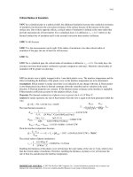
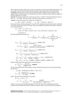
6-41
"!PROBLEM 6-41"
"GIVEN"
D=0.06 "[m]"
"N_dot=3000 rpm, parameter to be varied"
L_bearing=0.20 "[m]"
L=0.0002 "[m]"
T_0=50 "[C]"
"PROPERTIES"
k=0.17 "[W/m-K]"
mu=0.05 "[N-s/m^2]"
"ANALYSIS"
Vel=pi*D*N_dot*Convert(1/min, 1/s)
A=pi*D*L_bearing
T_max=T_0+(mu*Vel^2)/(8*k)

Q_dot=A*(mu*Vel^2)/(2*L)
W_dot_mech=Q_dot

N [rpm]
0
250
500
750
1000
1250
1500
1750
2000
2250
2500
2750
3000
3250
3500
3750
4000
4250
4500
4750
5000

Wmech [W]
0
2.907
11.63

26.16
46.51
72.67
104.7
142.4
186
235.5
290.7
351.7
418.6
491.3
569.8
654.1
744.2
840.1
941.9
1049
1163

6-15


Chapter 6 Fundamentals of Convection

1200

1000

W m ech [W ]

800

600

400

200

0
0

1000

2000

3000

N [rpm ]

6-16

4000

5000


Chapter 6 Fundamentals of Convection
6-42 A shaft rotating in a bearing is considered. The power required to rotate the shaft is to be determined
for different fluids in the gap.
Assumptions 1 Steady operating conditions exist. 2 The fluid has constant properties. 3 Body forces such

as gravity are negligible.
Properties The properties of air, water, and oil at 40°C are (Tables A-15, A-9, A-13)

Air:

μ = 1.918×10-5 N-s/m2

Water: μ = 0.653×10-3 N-s/m2
Oil:

2500 rpm

μ = 0.212 N-s/m2

12 m/s

Analysis A shaft rotating in a bearing can be
approximated as parallel flow between two large plates
with one plate moving and the other stationary.
Therefore, we solve this problem considering such a
flow with the plates separated by a L=0.5 mm thick
fluid film similar to the problem given in Example 6-1.
By simplifying and solving the continuity, momentum,
and energy equations it is found in Example 6-1 that

dT
W& mech = Q& 0 = −Q& L = −kA
dy

= −kA

y =0

5 cm

10 cm

2
2
μV 2
(1 − 0) = − A μV = − A μV
2kL
2L
2L

First, the velocity and the surface area are
⎛ 1 min ⎞
V = πDN& = π(0.05 m)(2500 rev/min )⎜
⎟ = 6.545 m/s
⎝ 60 s ⎠
A = πDL bearing = π(0.05 m)(0.10 m) = 0.01571 m 2

(a) Air:

(1.918 ×10 −5 N ⋅ s/m 2 )(6.545 m/s) 2
μV 2
W& mech = − A
= −(0.01571 m 2 )
2(0.0005 m)
2L

⎛ 1W ⎞
⎜
⎟ = −0.013 W
⎝ 1 N ⋅ m/s ⎠

(b) Water:

(0.653 ×10 −3 N ⋅ s/m 2 )(6.545 m/s) 2 ⎛ 1 W ⎞
μV 2
W& mech = Q& 0 = − A
= −(0.01571 m 2 )
⎜
⎟ = −0.44 W
2(0.0005 m)
2L
⎝ 1 N ⋅ m/s ⎠
(c) Oil:

(0.212 N ⋅ s/m 2 )(6.545 m/s) 2 ⎛ 1 W ⎞
μV 2
W& mech = Q& 0 = − A
= −(0.01571 m 2 )
⎜
⎟ = −142.7 W
2(0.0005 m)
2L
⎝ 1 N ⋅ m/s ⎠

6-17

Chapter 6 Fundamentals of Convection
6-43 The flow of fluid between two large parallel plates is considered. The relations for the maximum
temperature of fluid, the location where it occurs, and heat flux at the upper plate are to be obtained.
Assumptions 1 Steady operating conditions exist. 2 The fluid has constant properties. 3 Body forces such
as gravity are negligible.
Analysis We take the x-axis to be the flow direction, and y to be the normal direction. This is parallel flow
between two plates, and thus v = 0. Then the continuity equation reduces to
∂u ∂v
∂u
+
= 0 ⎯→
Continuity:
= 0 ⎯→ u = u(y)
V
∂x
∂x ∂y
Therefore, the x-component of velocity does not change
T0
in the flow direction (i.e., the velocity profile remains
unchanged). Noting that u = u(y), v = 0, and
L
Fluid
∂P / ∂x = 0 (flow is maintained by the motion of the
upper plate rather than the pressure gradient), the xmomentum equation reduces to
⎛ ∂u
∂u ⎞
∂ 2 u ∂P
d 2u
+ v ⎟⎟ = μ 2 −

⎯→
=0
x-momentum: ρ⎜⎜ u
∂y ⎠
∂x
∂y
dy 2
⎝ ∂x

This is a second-order ordinary differential equation, and integrating it twice gives
u ( y ) = C1 y + C 2

The fluid velocities at the plate surfaces must be equal to the velocities of the plates because of the no-slip
condition. Therefore, the boundary conditions are u(0) = 0 and u(L) = V , and applying them gives the
velocity distribution to be
u( y) =

y
V
L

Frictional heating due to viscous dissipation in this case is significant because of the high
viscosity of oil and the large plate velocity. The plates are isothermal and there is no change in the flow
direction, and thus the temperature depends on y only, T = T(y). Also, u = u(y) and v = 0. Then the energy
equation with dissipation (Eqs. 6-36 and 6-37) reduce to
2

⎛ ∂u ⎞
d 2T
⎛V⎞

⎜⎜ ⎟⎟
+
μ
⎯→
k
= −μ ⎜ ⎟
2
2
∂y
dy
⎝L⎠
⎝ ∂y ⎠
since ∂u / ∂y = V / L . Dividing both sides by k and integrating twice give
Energy:

0=k

∂ 2T

2

2

μ⎛V⎞
dT
= − ⎜ ⎟ y + C3
dy
k⎝L⎠
2

T ( y) = −

μ ⎛y ⎞
⎜ V⎟ + C3 y + C 4
2k ⎝ L ⎠

Applying the two boundary conditions give
dT
−k
=0⎯
⎯→ C 3 = 0
B.C. 1: y=0
dy y =0
B.C. 2: y=L

T ( L ) = T0 ⎯
⎯→ C 4 = T0 +

μV 2

2k
Substituting the constants give the temperature distribution to be

T ( y ) = T0 +

μV 2
2k

⎛ y2 ⎞
⎟

⎜1 −
⎜ L2 ⎟
⎠
⎝

The temperature gradient is determined by differentiating T(y) with respect to y,

6-18


Chapter 6 Fundamentals of Convection

dT − μV 2
y
=
dy
kL2
The location of maximum temperature is determined by setting dT/dy = 0 and solving for y,
dT − μV 2
=
y=0⎯
⎯→ y = 0
dy
kL2
Therefore, maximum temperature will occur at the lower plate surface, and it s value is

Tmax = T (0) = T0 +

μV 2
2k

.The heat flux at the upper plate is
q& L = −k

dT
dy

=k
y=L

μV 2
kL2

L=

μV 2
L

6-19


Chapter 6 Fundamentals of Convection
6-44 The flow of fluid between two large parallel plates is considered. Using the results of Problem 6-43, a
relation for the volumetric heat generation rate is to be obtained using the conduction problem, and the
result is to be verified.
Assumptions 1 Steady operating conditions exist. 2 The fluid has constant properties. 3 Body forces such
as gravity are negligible.
V
Analysis The energy equation in Prob. 6-44 was

determined to be
2
d 2T
⎛V⎞
μ
k
=
−
(1)
⎟
⎜
dy 2
⎝L⎠
L
Fluid
The steady one-dimensional heat conduction equation with
constant heat generation is
d 2 T g& 0
(2)
+
=0
k
dy 2
Comparing the two equation above, the volumetric heat generation rate is determined to be
2
⎛V⎞
g& 0 = μ ⎜ ⎟
⎝L⎠
Integrating Eq. (2) twice gives
g&

dT
= − 0 y + C3
dy
k
g& 0 2
y + C3 y + C4
T ( y) = −
2k

Applying the two boundary conditions give
dT
−k
=0⎯
⎯→ C 3 = 0
B.C. 1: y=0
dy y =0
g& 0 2
L
2k
Substituting, the temperature distribution becomes

B.C. 2: y=L

T ( L ) = T0 ⎯
⎯→ C 4 = T0 +

T ( y ) = T0 +

g& 0 L2
2k

⎛
y2 ⎞
⎜1 −
⎟
⎜
L2 ⎟⎠
⎝

Maximum temperature occurs at y = 0, and it value is
g& L2
Tmax = T (0) = T0 + 0
2k
which is equivalent to the result Tmax = T (0) = T0 +

μV 2
2k

6-20

obtained in Prob. 6-43.

T0


Chapter 6 Fundamentals of Convection
6-45 The oil in a journal bearing is considered. The bearing is cooled externally by a liquid. The surface
temperature of the shaft, the rate of heat transfer to the coolant, and the mechanical power wasted are to be
determined.
Assumptions 1 Steady operating conditions exist. 2 Oil is an incompressible substance with constant

properties. 3 Body forces such as gravity are negligible.
Properties The properties of oil are given to be k = 0.14 W/m-K and μ = 0.03 N-s/m2. The thermal
conductivity of bearing is given to be k = 70 W/m-K.
Analysis (a) Oil flow in a journal bearing can be approximated as parallel flow between two large plates
with one plate moving and the other stationary. We take the x-axis to be the flow direction, and y to be the
normal direction. This is parallel flow between two plates, and thus v = 0. Then the continuity equation
reduces to
∂u ∂v
∂u
+
= 0 ⎯→
Continuity:
= 0 ⎯→ u = u(y)
4500 rpm
∂x
∂x ∂y
Therefore, the x-component of velocity does not change
12 m/s
5 cm
in the flow direction (i.e., the velocity profile remains
unchanged). Noting that u = u(y), v = 0, and
∂P / ∂x = 0 (flow is maintained by the motion of the
upper plate rather than the pressure gradient), the xmomentum equation reduces to
15 cm
⎛ ∂u
∂u ⎞
∂ 2 u ∂P
d 2u
+ v ⎟⎟ = μ 2 −
⎯→

=0
x-momentum: ρ⎜⎜ u
∂y ⎠
∂x
∂y
dy 2
⎝ ∂x

This is a second-order ordinary differential equation, and integrating it twice gives
u ( y ) = C1 y + C 2

The fluid velocities at the plate surfaces must be equal to the velocities of the plates because of the no-slip
condition. Therefore, the boundary conditions are u(0) = 0 and u(L) = V , and applying them gives the
velocity distribution to be
u( y) =

y
V
L

where

⎛ 1 min ⎞
V = πDn& = π (0.05 m )(4500 rev/min)⎜
⎟ = 11.78 m/s
⎝ 60 s ⎠
The plates are isothermal and there is no change in the flow direction, and thus the temperature
depends on y only, T = T(y). Also, u = u(y) and v = 0. Then the energy equation with viscous dissipation
reduces to
2

2
⎛ ∂u ⎞
d 2T
⎛V⎞
0 = k 2 + μ⎜⎜ ⎟⎟
⎯→ k
Energy:
=
−
μ
⎜
⎟
∂y
dy 2
⎝L⎠
⎝ ∂y ⎠
since ∂u / ∂y =V / L . Dividing both sides by k and integrating twice give

∂ 2T

2

μ⎛V⎞
dT
= − ⎜ ⎟ y + C3
dy
k⎝L⎠
2

μ ⎛y ⎞
T ( y) = −
⎜ V⎟ + C3 y + C 4
2k ⎝ L ⎠
Applying the two boundary conditions give
dT
−k
=0⎯
⎯→ C 3 = 0
B.C. 1: y=0
dy y =0

6-21


Chapter 6 Fundamentals of Convection

B.C. 2: y=L

T ( L ) = T0 ⎯
⎯→ C 4 = T0 +

μV 2

2k
Substituting the constants give the temperature distribution to be

T ( y ) = T0 +

μV 2

2k

⎛ y2 ⎞
⎜1 −
⎟
⎜ L2 ⎟
⎝
⎠

The temperature gradient is determined by differentiating T(y) with respect to y,
dT − μV 2
y
=
dy
kL2
.The heat flux at the upper surface is

q& L = −k

dT
dy

=k
y=L

μV 2
kL2

L=

μV 2
L

Noting that heat transfer along the shaft is negligible, all the heat generated in the oil is transferred to the
shaft, and the rate of heat transfer is
(0.03 N ⋅ s/m 2 )(11.78 m/s) 2
μV 2
Q& = As q& L = (πDW )
= π (0.05 m)(0.15 m)
= 163.5 W
L
0.0006 m
(b) This is equivalent to the rate of heat transfer through the cylindrical sleeve by conduction, which is
expressed as

2πW (T0 − Ts )
Q& = k
ln( D0 / D )

→ (70 W/m ⋅ °C)

2π (0.15 m)(T0 - 40°C)
= 163.5 W
ln(8 / 5)

which gives the surface temperature of the shaft to be
To = 41.2°C
(c) The mechanical power wasted by the viscous dissipation in oil is equivalent to the rate of heat generation,
W& lost = Q& = 163.5 W

6-22


Chapter 6 Fundamentals of Convection
6-46 The oil in a journal bearing is considered. The bearing is cooled externally by a liquid. The surface
temperature of the shaft, the rate of heat transfer to the coolant, and the mechanical power wasted are to be
determined.
Assumptions 1 Steady operating conditions exist. 2 Oil is an incompressible substance with constant
properties. 3 Body forces such as gravity are negligible.
Properties The properties of oil are given to be k = 0.14 W/m-K and μ = 0.03 N-s/m2. The thermal
conductivity of bearing is given to be k = 70 W/m-K.
Analysis (a) Oil flow in a journal bearing can be approximated as parallel flow between two large plates
with one plate moving and the other stationary. We take the x-axis to be the flow direction, and y to be the
normal direction. This is parallel flow between two plates, and thus v = 0. Then the continuity equation
reduces to
∂u ∂v
∂u
+
= 0 ⎯→
Continuity:
= 0 ⎯→ u = u(y)
4500 rpm
∂x
∂x ∂y
Therefore, the x-component of velocity does not change
12 m/s
5 cm
in the flow direction (i.e., the velocity profile remains
unchanged). Noting that u = u(y), v = 0, and
∂P / ∂x = 0 (flow is maintained by the motion of the

upper plate rather than the pressure gradient), the xmomentum equation reduces to
15 cm
⎛ ∂u
∂u ⎞
∂ 2 u ∂P
d 2u
+ v ⎟⎟ = μ 2 −
⎯→
=0
x-momentum: ρ⎜⎜ u
∂y ⎠
∂x
∂y
dy 2
⎝ ∂x

This is a second-order ordinary differential equation, and integrating it twice gives
u ( y ) = C1 y + C 2

The fluid velocities at the plate surfaces must be equal to the velocities of the plates because of the no-slip
condition. Therefore, the boundary conditions are u(0) = 0 and u(L) = V , and applying them gives the
velocity distribution to be
u( y) =

y
V
L

where

⎛ 1 min ⎞
V = πDn& = π (0.05 m )(4500 rev/min)⎜
⎟ = 11.78 m/s
⎝ 60 s ⎠
The plates are isothermal and there is no change in the flow direction, and thus the temperature
depends on y only, T = T(y). Also, u = u(y) and v = 0. Then the energy equation with viscous dissipation
reduces to
2

2
⎛ ∂u ⎞
d 2T
⎛V⎞
0 = k 2 + μ⎜⎜ ⎟⎟
⎯→ k
Energy:
=
−
μ
⎜
⎟
∂y
dy 2
⎝L⎠
⎝ ∂y ⎠
since ∂u / ∂y =V / L . Dividing both sides by k and integrating twice give

∂ 2T

2

μ⎛V⎞
dT
= − ⎜ ⎟ y + C3
dy
k⎝L⎠
2

μ ⎛y ⎞
T ( y) = −
⎜ V⎟ + C3 y + C 4
2k ⎝ L ⎠
Applying the two boundary conditions give
dT
−k
=0⎯
⎯→ C 3 = 0
B.C. 1: y=0
dy y =0

6-23


Chapter 6 Fundamentals of Convection

B.C. 2: y=L

T ( L ) = T0 ⎯
⎯→ C 4 = T0 +

μV 2

2k
Substituting the constants give the temperature distribution to be

T ( y ) = T0 +

μV 2
2k

⎛ y2 ⎞
⎜1 −
⎟
⎜ L2 ⎟
⎝
⎠

The temperature gradient is determined by differentiating T(y) with respect to y,
dT − μV 2
y
=
dy
kL2
.The heat flux at the upper surface is

q& L = −k

dT
dy

=k
y=L

μV 2
kL2

L=

μV 2
L

Noting that heat transfer along the shaft is negligible, all the heat generated in the oil is transferred to the
shaft, and the rate of heat transfer is
(0.03 N ⋅ s/m 2 )(11.78 m/s) 2
μV 2
Q& = As q& L = (πDW )
= π (0.05 m)(0.15 m)
= 98.1 W
L
0.001 m
(b) This is equivalent to the rate of heat transfer through the cylindrical sleeve by conduction, which is
expressed as

2πW (T0 − Ts )
Q& = k
ln( D0 / D )

→ (70 W/m ⋅ °C)

2π (0.15 m)(T0 - 40°C)

= 98.1 W
ln(8 / 5)

which gives the surface temperature of the shaft to be
To = 40.7°C
(c) The mechanical power wasted by the viscous dissipation in oil is equivalent to the rate of heat generation,
W& lost = Q& = 98.1 W

6-24


Chapter 6 Fundamentals of Convection

Momentum and Heat Transfer Analogies

6-47C Reynolds analogy is expressed as C f , x

Re L
= Nu x . It allows us to calculate the heat transfer
2

coefficient from a knowledge of friction coefficient. It is limited to flow of fluids with a Prandtl number of
near unity (such as gases), and negligible pressure gradient in the flow direction (such as flow over a flat
plate).

Modified

6-48C

C f ,x

2

=

Reynolds

analogy

is

expressed

as

C f ,x

Re L
= Nu x Pr −1 / 3
2

or

hx
Pr 2/3 ≡ j H . It allows us to calculate the heat transfer coefficient from a knowledge of
ρC pV

friction coefficient. It is valid for a Prandtl number range of 0.6 < Pr < 60. This relation is developed using
relations for laminar flow over a flat plate, but it is also applicable approximately for turbulent flow over a
surface, even in the presence of pressure gradients.
6-49 A flat plate is subjected to air flow, and the drag force acting on it is measured. The average

convection heat transfer coefficient and the rate of heat transfer are to be determined.
Assumptions 1 Steady operating conditions exist. 2 The edge effects are negligible.

Air
20°C
10 m/s

Properties The properties of air at 20°C and 1 atm are (Table A-15)

ρ = 1.204 kg/m3,

Cp =1.007 kJ/kg-K,

Pr = 0.7309

Analysis The flow is along the 4-m side of the plate, and thus the
characteristic length is L = 4 m. Both sides of the plate is exposed to
air flow, and thus the total surface area is

L=4 m

As = 2WL = 2(4 m)(4 m) = 32 m 2
For flat plates, the drag force is equivalent to friction force. The
average friction coefficient Cf can be determined from
F f = C f As

ρV 2
2

⎯

⎯→ C f =

Ff
ρA s V / 2
2

=

⎛ 1 kg ⋅ m/s 2
⎜
1N
(1.204 kg/m 3 )(32 m 2 )(10 m/s) 2 / 2 ⎜⎝
2. 4 N

⎞
⎟ = 0.006229
⎟
⎠

Then the average heat transfer coefficient can be determined from the modified Reynolds analogy to be
h=

C f ρV C p

=

0.006229 (1.204 kg/m 3 )(10 m/s)(1007 J/kg ⋅ °C)
= 46.54 W/m 2 ⋅ C
2
/

3
2
(0.7309)

Pr 2/3
Them the rate of heat transfer becomes
Q& = hA (T − T ) = (46.54 W/m 2 ⋅ °C)(32 m 2 )(80 − 20)°C = 89,356 W
2

s

s

∞

6-25