Deep Learning for the Life Sciences: Applying Deep Learning to Genomics, Microscopy, Drug Discovery, and More
Bạn đang xem bản rút gọn của tài liệu. Xem và tải ngay bản đầy đủ của tài liệu tại đây (4.61 MB, 82 trang )
History
Deep Learning for the Life Sciences
Topics
Bharath Ramsundar, Peter Eastman, Karl Leswing, Patrick Walters, and Vijay Pande
Tutorials
Offers & Deals
Highlights
Settings
Support
Sign Out
Playlists
Deep Learning for the Life Sciences
History
by Bharath Ramsundar , Karl Leswing , Peter Eastman , and Vijay Pande
Topics
Copyright © 2019 Bharath Ramsundar, Karl Leswing, Peter Eastman, and Vijay Pande. All
rights reserved.
Tutorials
Printed in the United States of America.
Offers & Deals
Published by O’Reilly Media, Inc., 1005 Gravenstein Highway North, Sebastopol, CA 95472.
Highlights
O’Reilly books may be purchased for educational, business, or sales promotional use. Online
Settings
editions are also available for most titles ( />
contact our corporate/institutional sales department: 8009989938 or
Support
Sign Out
Acquisitions Editor: Mike Loukides
Developmnent Editor: Nicole Tache
Production Editor: Justin Billing
Interior Designer: David Futato
Cover Designer: Karen Montgomery
Illustrator: Rebecca Demarest
April 2019: First Edition
Revision History for the Early Release
20181126: First Release
See />The O Reilly logo is a registered trademark of O Reilly Media, Inc. Deep Learning for the Life
Sciences, the cover image, and related trade dress are trademarks of O’Reilly Media, Inc.
The views expressed in this work are those of the authors, and do not represent the publisher’s
views. While the publisher and the authors have used good faith efforts to ensure that the
information and instructions contained in this work are accurate, the publisher and the authors
disclaim all responsibility for errors or omissions, including without limitation responsibility for
damages resulting from the use of or reliance on this work. Use of the information and
instructions contained in this work is at your own risk. If any code samples or other technology
this work contains or describes is subject to open source licenses or the intellectual property
rights of others, it is your responsibility to ensure that your use thereof complies with such
licenses and/or rights.
9781492039761
[LSI]
Chapter 1. Machine Learning with
DeepChem
Topics
History
Tutorials
A NOTE REGARDING EARLY RELEASE CHAPTERS
Offers & Deals
Thank you for investing in the Early Release version of this book! Note that
Highlights
“Machine Learning with DeepChem” is going to be Chapter 3 in the final book.
Settings
This chapter provides a brief introduction to machine learning with DeepChem. DeepChem is a
Support
library built on top of the TensorFlow platform to facilitate the use of deep learning in the life
Signsciences. DeepChem provides a large collection of models, algorithms, and datasets that are
Out
suited to applications in the life sciences. In the remainder of this book, we will use DeepChem
in order to perform our case studies.
WHY NOT JUST USE KERAS OR TENSORFLOW OR
PYTORCH?
A common question for DeepChem developers is why not just use Keras or
TensorFlow or PyTorch? The short answer is that the developers of these packages
focus their attention on supporting certain types of use cases that prove useful to
their core users. For example, there’s extensive support for image processing, text
handling, and speech analysis. But there’s often not similar levels of support in
these libraries for molecule handling, genetic datasets, or microscopy datasets. The
goal of DeepChem is to give these applications first class support in the library.
This means adding custom deep learning primitives, support for needed filetypes,
and extensive tutorials and documentation for these use cases.
DeepChem is also designed to be well integrated with the TensorFlow ecosystem,
so you should be able to mix and match DeepChem code with your other
TensorFlow application code.
DeepChem Datasets
DeepChem uses the basic abstraction of the Dataset object to wrap the data it uses for
machine learning. A Dataset contains the information about a set of samples: the input
vectors , the target output vectors , and possibly other information such as a description of
what each sample represents. There are subclasses of Dataset corresponding to different
ways of storing the data. The NumpyDataset object in particular serves as a convenient
wrapper for NumPy arrays and will be used extensively. In this section, we will walk through a
simple code case study of how to use NumpyDataset. We start with some simple imports.
import deepchem as dc
import numpy as np
Let’s now construct some simple NumPy arrays.
x = np.random.random((4, 5))
y = np.random.random((4, 1))
This dataset will have four samples. The array x has five elements (“features”) for each sample,
and y has 1 element for each sample. Let’s take a quick look at the actual arrays we’ve sampled.
(Note that when you run this code locally, you should expect to see different numbers since your
random seed will be different).
In: x
Out:
array([[0.960767 , 0.31300931, 0.23342295, 0.59850938, 0.30457302],
[0.48891533, 0.69610528, 0.02846666, 0.20008034, 0.94781389],
[0.17353084, 0.95867152, 0.73392433, 0.47493093, 0.4970179 ],
[0.15392434, 0.95759308, 0.72501478, 0.38191593, 0.16335888]])
In: y
Out:
array([[0.00631553],
[0.69677301],
[0.16545319],
[0.04906014]])
Let’s now wrap these arrays in a NumpyDataset object.
dataset = dc.data.NumpyDataset(x, y)
We can “unwrap” the dataset object to get at the original arrays that we stored inside.
In: print(dataset.X)
[[0.960767 0.31300931 0.23342295 0.59850938 0.30457302]
[0.48891533 0.69610528 0.02846666 0.20008034 0.94781389]
[0.17353084 0.95867152 0.73392433 0.47493093 0.4970179 ]
[0.15392434 0.95759308 0.72501478 0.38191593 0.16335888]]
In: print(dataset.y)
[[0.00631553]
[0.69677301]
[0.16545319]
[0.04906014]]
Note that these arrays are the same as the original arrays x and y.
In [23]: np.array_equal(x, dataset.X)
Out[23]: True
In [24]: np.array_equal(y, dataset.y)
Out[24]: True
OTHER TYPES OF DATASETS
DeepChem has support for other types of Dataset as mentioned previously.
These types of Dataset objects primarily become useful when dealing with larger
datasets that can’t be entirely stored in computer memory. There is also integration
for DeepChem to use TensorFlow’s tf.data dataset loading utilities. We will
touch on these more advanced library features as we need them.
Training a Model to Predict Toxicity of Molecules
In this section, we will learn how to use DeepChem to train a model to predict the toxicity of
molecules. In a later chapter, we will explain how toxicity prediction for molecules works in
much greater depth, but in this section, we will treat it as a black box example of how
DeepChem models can be used to solve machine learning challenges. Let’s start with a pair of
needed imports.
import numpy as np
import deepchem as dc
The next step is loading the associated toxicity datasets for training a machine learning model.
DeepChem maintains a module dc.molnet (short for MoleculeNet) that contains a number of
preprocessed datasets for use in machine learning experimentation. In particular, we will make
use of the dc.molnet.load_tox21() function which will load and process the Tox21
toxicity dataset for us. When you run these commands for the first time, DeepChem will process
the dataset locally on your machine. You should expect to see processing notes like the
following.
In : tox21_tasks, tox21_datasets, transformers = dc.molnet.load_tox21()
Loading raw samples now.
shard_size: 8192
About to start loading CSV from /tmp/tox21.csv.gz
Loading shard 1 of size 8192.
Featurizing sample 0
Featurizing sample 1000
Featurizing sample 2000
Featurizing sample 3000
Featurizing sample 4000
Featurizing sample 5000
Featurizing sample 6000
Featurizing sample 7000
TIMING: featurizing shard 0 took 15.671 s
TIMING: dataset construction took 16.277 s
Loading dataset from disk.
TIMING: dataset construction took 1.344 s
Loading dataset from disk.
TIMING: dataset construction took 1.165 s
Loading dataset from disk.
TIMING: dataset construction took 0.779 s
Loading dataset from disk.
TIMING: dataset construction took 0.726 s
Loading dataset from disk.
The process of featurization is how a dataset containing information about molecules is
transformed into matrices and vectors for use in machine learning analyses. We will explore the
process of featurization in greater depth in subsequent chapters. Let’s start here though by
taking a quick peek at the data we’ve processed. The dc.molnet.load_tox21() function
returns multiple outputs: tox21_tasks, tox21_datasets, and transformers. Let’s
briefly take a look at each.
In : tox21_tasks
Out:
['NRAR',
'NRARLBD',
'NRAhR',
'NRAromatase',
'NRER',
'NRERLBD',
'NRPPARgamma',
'SRARE',
'SRATAD5',
'SRHSE',
'SRMMP',
'SRp53']
In : len(tox21_tasks)
Out: 12
Each of these 12 tasks here corresponds to a particular biological experiment. In this case, each
of these tasks is for an enzymatic assay which measures whether the molecules in the Tox21
dataset bind with the biological target in question. The terms ‘NRAR’ and other above
correspond with these targets. In this case, each of these targets is a particular enzyme believed
to be linked to toxic responses to potential therapeutic molecules.
HOW MUCH BIOLOGY DO I NEED TO KNOW?
For computer scientists and engineers entering the life sciences, the array of
biological terms can be dizzying. However, it’s not necessary to have a deep
understanding of biology in order to begin making an impact in the life sciences. If
your primary background is in computer science, it can be useful to try
understanding biological systems in terms of computer scientific analogues.
Imagine that cells or animals are complex legacy codebases that you have no
control over. As an engineer, you have a few experimental measurements of these
systems (assays) which you can use to gain some understanding of the underlying
mechanics of the system. Machine learning is an extraordinarily powerful tool for
understanding biological systems since learning algorithms are capable of extracting
useful correlations in a mostly automatic fashion. This allows even biological
beginners to sometimes find deep biological insights.
In the remainder of this book, we shall discuss basic biology in brief asides. These
notes can serve as starting points into the vast biological literature. Public references
such as Wikipedia often contain a wealth of useful information, and can help
bootstrap your biological education.
Next, let’s consider tox21_datasets. The use of the plural is a clue that this field is actually
a tuple containing multiple dc.data.Dataset objects:
In : tox21_datasets
Out:
(<deepchem.data.datasets.DiskDataset at 0x7f9804d6c390>,
<deepchem.data.datasets.DiskDataset at 0x7f9804d6c780>,
<deepchem.data.datasets.DiskDataset at 0x7f9804c5a518>)
In this case, these datasets correspond to the training, validation, and test set you learned about
in the previous chapter. You might note that these are DiskDataset objects; the dc.molnet
module caches these datasets on your disk so that you don’t need to repeatedly refeaturize the
Tox21 dataset. Let’s split up these datasets correctly.
train_dataset, valid_dataset, test_dataset = tox21_datasets
When dealing with new datasets, it’s very useful to start by taking a look at their shapes. To do
so, inspect the shape attribute.
In : train_dataset.X.shape
Out: (6264, 1024)
In : valid_dataset.X.shape
Out: (783, 1024)
In : test_dataset.X.shape
Out: (784, 1024)
The train_dataset contains a total of 6264 samples, each of which has an associated
feature vector of length 1024. Similarly, valid_dataset and test_dataset contain
respectively 783 and 784 samples. Let’s now take a quick look at the vectors for these
datasets.
In : np.shape(train_dataset.y)
Out: (6264, 12)
In : np.shape(valid_dataset.y)
Out: (783, 12)
In : np.shape(test_dataset.y)
Out: (784, 12)
There are 12 data points, also known as labels, for each sample. These correspond to the 12
tasks we discussed above. In this particular dataset, the samples correspond to molecules, the
tasks correspond to biochemical assays, and each label is the result of a particular assay on a
particular molecule. Those are what we want to train our model to predict.
There’s a complication, however. The actual experimental dataset for Tox21 did not test every
molecule in every biological experiment. That means that some of these labels are meaningless
placeholders. We simply don’t have any data for some properties of some molecules, so we
need to ignore those elements of the arrays when training and testing the model.
How can we find which labels were actually measured? We can check the dataset’s w field,
which records its weights. Whenever we compute the loss function for a model, we multiply by
w before summing over tasks and samples. This can be used for a few purposes, one being to
flag missing data. If a label has a weight of 0, that label does not affect the loss and is ignored
during training. Let’s do some digging to find how many labels have actually been measured in
our datasets.
In [37]: train_dataset.w.shape
Out[37]: (6264, 12)
In [38]: np.count_nonzero(train_dataset.w)
Out[38]: 62166
In [39]: np.count_nonzero(train_dataset.w == 0)
Out[39]: 13002
So of the 6264 × 12 = 75,168 elements in the array of labels, only 62,166 were actually
measured. The other 13,002 correspond to missing measurements and should be ignored. You
might ask then why we still keep such entries around. The answer is mainly for convenience;
irregularly shaped arrays are much harder to reason about and deal with in code than regular
matrices with an associated set of weights.
PROCESSING DATASETS IS CHALLENGING
It’s important to note here that cleaning and processing a dataset for use in the life
sciences can be extremely challenging. Many raw datasets will contain systematic
classes of errors. If the dataset in question has been constructed from an experiment
conducted by an external organization (a “Contract Research Organization” or
CRO), it’s quite possible that the dataset will be systematically wrong. For this
reason, many life science organizations maintain scientists inhouse whose job it is
to verify and clean such datasets.
In general, if your machine learning algorithm isn’t working for a life science task,
there’s a significant chance that the root cause stems not from the algorithm but
from systematic errors in the source of data that you’re using.
Now let’s examine transformers, the final output that was returned by load_tox21().
A transformer is an object that modifies a dataset in some way. DeepChem provides many
transformers that manipulate data in useful ways. The data loading routines found in
MoleculeNet always return a list of transformers that have been applied to the data, since you
may need them later to “untransform” the data. Let’s see what we have in this case.
In [2]: transformers
Out[2]: [<deepchem.trans.transformers.BalancingTransformer at 0x7f99dd73c6d8>]
The data has been transformed with a BalancingTransformer. This class is used to
correct for unbalanced data. In the case of Tox21, most molecules do not bind to most of the
targets. In fact, over 90% of the labels are 0. That means a model could trivially achieve over
90% accuracy simply by always predicting 0, no matter what input it was given. Unfortunately,
that model would be completely useless! Unbalanced data, where there are many more training
samples for some classes than others, is a common problem in classification tasks.
Fortunately, there is an easy solution: adjust the dataset’s matrix of weights to compensate.
BalancingTransformer adjusts the weights for individual data points so that the total
weight assigned to every class is the same. That way, the loss function has no systematic
preference for any one class. The loss can only be decreased by learning to correctly distinguish
between classes.
Now that we’ve explored the Tox21 datasets, let’s start exploring how we can train models on
these datasets. DeepChem’s dc.models submodule contains a variety of different lifescience
specific models. All of these various models inherit from the parent class
dc.models.Model. This parent class is designed to provide a common API that follows
common Python conventions. If you’ve used other Python machine learning packages, you
should find that many of dc.models.Model methods look quite familiar.
In this chapter, we won’t really dig into the details of how these models are constructed. Rather,
we will just provide an example of how to instantiate a standard DeepChem model,
dc.models.MultitaskClassifier. This model builds a fully connected network (a
MLP) that maps input features to multiple output predictions. This makes it useful for multitask
problems, where there are multiple labels for every sample. It’s well suited for our Tox21
datasets, since we have a total of 12 different assays we wish to predict simultaneously. Let’s
see how we can construct a MultitaskClassifier in DeepChem.
model = dc.models.MultitaskClassifier(n_tasks=12,
n_features=1024,
layer_sizes=[1000])
There are a variety of different options here. Let’s briefly review them. n_tasks is the number
of tasks, and n_features is the number of input features for each sample. As we saw above,
the Tox21 dataset has 12 tasks and 1024 features for each sample. layer_sizes is a list that
sets the number of fully connected hidden layers in the network, and the width of each one. In
this case, we specify that there is a single hidden layer of width 1000.
Now that we’ve constructed the model, how can we train it on the Tox21 datasets? Each Model
object has a fit() method that fits the model to the data contained in a Dataset object.
Fitting our MultitaskClassifier object is a simple call then.
model.fit(train_dataset, nb_epoch=10)
Note that we added on a flag here. nb_epoch=10 says that 10 epochs of gradient descent
training will be conducted. An epoch refers to one complete pass through all the samples in a
dataset. To train a model, you divide the training set into batches and take one step of gradient
descent for each batch. In an ideal world, you would reach a well optimized model before
running out of data. In practice, there usually isn’t enough training data for that, so you run out
of data before the model is fully trained. You then need to start reusing data, making additional
passes through the dataset. This lets you train models with smaller amounts of data, but the
more epochs you use, the more likely you are to end up with an overfit model.
Let’s now evaluate the performance of the trained model. In order to evaluate how well a model
works, it is necessary to specify a metric. The DeepChem class dc.metrics.Metric
provides a general way to specify metrics for models. For Tox21 datasets, the ROCAUC score
is a useful metric, so let’s do our analysis using it. However, note a subtlety here: there are
multiple Tox21 tasks. Which one do we compute the ROCAUC on? A good tactic is to
compute the mean ROCAUC across all tasks. Luckily, it’s easy to do this
metric = dc.metrics.Metric(dc.metrics.roc_auc_score, np.mean)
ROCAUC
We want to classify molecules as toxic or nontoxic, but the model outputs
continuous numbers, not discrete predictions. In practice you pick a threshold value
and predict that a molecule is toxic whenever the output is greater than the
threshold. A low threshold will produce many false positives (predicting a safe
molecule is actually toxic). A higher threshold will give fewer false positives but
more false negatives (incorrectly predicting that a toxic molecule is safe).
The receiver operating characteristic (ROC) curve is a convenient way to visualize
this tradeoff. You try many different threshold values, then plot a curve of the true
positive rate versus the false positive rate as the threshold is varied. An example is
shown in Figure 31.
The ROCAUC is the total area under the ROC curve. If there exists any threshold
value for which every sample is classified correctly, the ROCAUC is 1. At the
other extreme, if the model outputs completely random values unrelated to the true
classes, the ROCAUC is 0.5. This makes it a useful number for summarizing how
well a classifier works. It’s just a heuristic, but it’s a popular one.
Since we’ve specified np.mean, the mean of the ROCAUC across all tasks will be reported.
DeepChem models support the evaluation function Model.evaluate() which evaluates the
performance of the model on a given dataset and metric.
train_scores = model.evaluate(train_dataset, [metric], transformers)
test_scores = model.evaluate(test_dataset, [metric], transformers)
Now that we’ve calculated the scores, let’s take a look!
In : print(train_scores)
...: print(test_scores)
...:
{'meanroc_auc_score': 0.9659541853946179}
{'meanroc_auc_score': 0.7915464001982299}
Notice that our score on the training set (0.96) is much better than our score on the test set
(0.79). This shows the model has been overfit. The test set score is the one we really care
about. These numbers aren’t the best possible on this dataset. At the time of writing, the best
numbers on the Tox21 dataset are a little under 0.9 mean ROCAUC. At the same time, these
numbers aren’t bad at all for an out of the box system. The complete ROC curve for one of the
12 tasks is shown in Figure 31.
Figure 11. The ROC curve for one of the 12 tasks. The dotted diagonal line shows what the curve would
be for a model that just guessed at random. The actual curve is consistently well above the diagonal,
showing that we are doing much better than random guessing.
Case Study: Training a MNIST Model
In the previous section, we covered the basics of training a machine learning model with
DeepChem. However, we used a premade model class
dc.models.MultitaskClassifier. Sometimes you may want to create a new deep
learning architecture instead of using a preconfigured one. In this section, we discuss how to
train a convolutional neural network on the MNIST digit recognition dataset. Instead of using a
premade architecture like in the previous example, this time we will specify the full deep
learning architecture ourselves. To do so, we will introduce the dc.models.TensorGraph
class which provides a framework for building deep architectures in DeepChem.
MNIST Digit Recognition Dataset
The MNIST image recognition dataset (see Figure 32) requires the construction of a machine
learning model that can learn to classify handwritten digits correctly. The challenge is to
classify digits from 0 to 9 given 28x28 pixel black and white images. The dataset contains
60,000 training examples and a test set of 10,000 examples.
Figure 12. Samples drawn from the MNIST handwritten digit recognition dataset. Source: Josef
Steppan />
The MNIST dataset is not particularly challenging as far as machine learning problems go.
Decades of research have produced state of the art algorithms that achieve close to 100% test set
accuracy on this dataset. As a result, the MNIST dataset is no longer suitable for research work,
but is a good tool for pedagogical purposes.
ISN’T DEEPCHEM JUST FOR THE LIFE SCIENCES?
As we mentioned earlier in the chapter, it’s entirely feasible to do life science
applications using other deep learning packages. Similarly, it’s quite feasible to
build general machine learning systems using DeepChem. Although building a
movie recommendation system in DeepChem might be trickier than it would be
with more specialized tools, it would be quite feasible to do so. And for good
reason: there have been multiple studies looking into the use of recommendation
system algorithms for use in molecular binding prediction. Machine learning
architectures used in one field tend to carry over to other fields, so it’s important to
retain the flexibility needed for innovative work.
A Convolutional Architecture for MNIST
DeepChem uses the TensorGraph class to construct nonstandard deep learning architectures.
In this section, we will walk through the code required to construct the convolutional
architecture shown in Figure 33. It begins with two convolutional layers to identify local
features within the image. They are followed by two fully connected layers to predict the digit
from those local features.
Figure 13. This diagram illustrates the architecture that we will construct in this section for processing
the MNIST architecture (Source: />processingforneuralcaseTabikPeralta/bb885ce41effcdfaee1f33dc084c029284850cab
Let’s start by downloading the raw MNIST data files locally.
mkdir MNIST_data
cd MNIST_data
wget />wget />wget />
wget />cd ..
Once you’ve executed these commands, you will have downloaded the MNIST dataset locally
and stored it. Let’s now load these datasets.
from tensorflow.examples.tutorials.mnist import input_data
mnist = input_data.read_data_sets("MNIST_data/", one_hot=True)
We’re going to process this raw data into a format suitable for analysis by DeepChem. Let’s
start by making the necessary imports.
import deepchem as dc
import tensorflow as tf
import deepchem.models.tensorgraph.layers as layers
The submodule deepchem.models.tensorgraph.layers contains a collection of
“layers.” These layers serve as building blocks of deep architectures and can be composed
together to build new deep learning architectures. We will demonstrate how layer objects are
used shortly. We now construct NumpyDataset objects that wrap the MNIST training and
test datasets.
train_dataset = dc.data.NumpyDataset(mnist.train.images, mnist.train.l
abels)
test_dataset = dc.data.NumpyDataset(mnist.test.images, mnist.test.labe
ls)
Note that although there wasn’t originally a test dataset defined, the input_data function
from TensorFlow takes care of separating out a proper test dataset for our use. With the training
and test datasets in hand, we can now turn our attention towards defining the architecture for the
MNIST convolutional network.
The key concept this is based on is that layer objects can be composed to build new models. As
we discussed in the previous chapter, each layer takes input from previous layers and computes
an output that can be passed to subsequent layers. At the very start, there are input layers that
take in features and labels. At the other end are output layers that return the results of the
performed computation. In this example, we will compose a sequence of layers in order to
construct an image processing convolutional network. We first start by defining a
new TensorGraph object.
model = dc.models.TensorGraph(model_dir='mnist')
The model_dir option specifies a directory where the model’s parameters should be saved.
You can omit this, as we did in the previous example, but then the model will not be saved. As
soon as the Python interpreter exits, all your hard work training the model will be thrown out!
By specifying a directory, you can reload the model later and make new predictions with it.
Note that since TensorGraph inherits from Model, this object is an instance of
dc.models.Model and supports the same fit() and evaluate() functions we saw
previously.
In : isinstance(model, dc.models.Model)
Out: True
We haven’t added anything to model yet, so our model isn’t likely to be very interesting. Let’s
start by adding some inputs for features and labels by using the Feature and Label classes.
feature = layers.Feature(shape=(None, 784))
label = layers.Label(shape=(None, 10))
MNIST contains images of size 28×28. When flattened, these form feature vectors of length
784. The labels have second dimension 10 since there are 10 possible digit values, and the
vector is onehot encoded. Note that None is used as an input dimension. In systems that build
on TensorFlow, the value None often encodes the ability for a given layer to accept inputs that
have any size in that dimension. Put another way, our object feature is capable of accepting
inputs of shape (20, 784) and (97, 784) with equal facility. In this case, the first
dimension corresponds to the batch size, so our model will be able to accept batches with any
number of samples.
ONEHOT ENCODING
The MNIST dataset is categorical. That is, objects belong to one of a finite list of
potential categories. In this case, these categories are the digits 0 through 9. How
can we feed these categories into a machine learning system? One obvious answer
would be to simply feed in a single number that takes values from 0 through 9.
However, for a variety of technical reasons, this encoding often doesn’t seem to
work well. The alternative that people often use is to onehot encode. Each label for
MNIST is a vector of length 10 in which a single element is set to 1, and all others
are set to zero. If the nonzero value is at the 0th index, then the label corresponds to
digit 0. If the nonzero value is at the 9th index, then the label corresponds to digit 9.
In order to apply convolutional layers to our input, we need to convert our flat feature vectors
into matrices of shape (28, 28). To do this, we will use a Reshape layer.
make_image = layers.Reshape(shape=(None, 28, 28), in_layers=feature)
Here again the value None indicates that arbitrary batch sizes can be handled. Note that we
have a keyword argument in_layers=feature. This indicates that the Reshape layer
takes our previous Feature layer feature as input. Now that we have successfully reshaped
the input, we can pass it through to the convolutional layers.
conv2d_1 = layers.Conv2D(num_outputs=32, activation_fn=tf.nn.relu, in_layers=mak
conv2d_2 = layers.Conv2D(num_outputs=64, activation_fn=tf.nn.relu, in_layers=con
Here the Conv2D class applies a two dimensional convolution to each sample of its input, then
passes it through a rectified linear unit (ReLU) activation function. Note how in_layers is
used to pass along previous layers as inputs to succeeding layers. We want to end by applying
Dense (fully connected) layers to the outputs of the convolutional layer. However, the output
of Conv2D layers is two dimensional, so we will first need to apply a Flatten layer to flatten
our input to one dimension. (More precisely, the Conv2D layer produces a two dimensional
output for each sample, so its output has three dimensions. The Flatten layer collapses this
to a single dimension per sample, or two dimensions in total.)
flatten = layers.Flatten(in_layers=conv2d_2)
dense1 = layers.Dense(out_channels=1024, activation_fn=tf.nn.relu, in_layers=fla
dense2 = layers.Dense(out_channels=10, activation_fn=None, in_layers=dense1)
The out_channels argument in a Dense layer specifies the width of the layer. The first
layer outputs 1024 values per sample, but the second layer outputs 10 values, corresponding to
our 10 possible digit values. We now want to hook this output up to a loss function, so we can
train the output to accurately predict classes. We will use the SoftMaxCrossEntropy loss
to perform this form of training.
smce = layers.SoftMaxCrossEntropy(in_layers=[label, dense2])
loss = layers.ReduceMean(in_layers=smce)
model.set_loss(loss)
Note that the SoftMaxCrossEntropy layer accepts both the labels and the output of the last
Dense layer as inputs. It computes the value of the loss function for every sample, so we then
need to average over all samples to obtain the final loss. This is done with the ReduceMean
layer, which we set as our model’s loss function by calling model.set_loss().
SOFTMAX AND SOFTMAXCROSSENTROPY
You often want a model to output a probability distribution. For MNIST, we want
to output the probability that a given sample represents each of the ten digits. Every
output must be positive, and they must add to 1. An easy way to achieve this is to
let the model compute arbitrary numbers, then pass them through the confusingly
named softmax function:
. The exponential in the numerator ensures
that all values are positive, and the sum in the denominator ensures they add to 1. If
one element of is much larger than the others, the corresponding output element
is very close to 1 and all other outputs are very close to 0.
SoftMaxCrossEntropy first uses a softmax to convert the outputs to probabilities,
then computes the cross entropy of those probabilities with the labels. Remember
that the labels are onehot encoded: 1 for the correct class, 0 for all others. You can
think of that as a probability distribution! The loss is minimized when the predicted
probability of the correct class is as close to 1 as possible. These two operations
(softmax followed by cross entropy) often appear together, and computing them as a
single step turns out to be more numerically stable than performing them separately.
For numerical stability, layers like SoftMaxCrossEntropy compute in logprobabilities.
We will need to transform the output with a SoftMax layer to obtain perclass output
probabilities. We will add this output to model with model.add_output().
output = layers.SoftMax(in_layers=dense2)
model.add_output(output)
We can now train the model using the same fit() function we called in the previous section.
model.fit(train_dataset, nb_epoch=10)
Let’s define our metric this time to be accuracy, the fraction of labels that are correctly
predicted.
metric = dc.metrics.Metric(dc.metrics.accuracy_score)
We can then compute the accuracy using the same computation as before.
train_scores = model.evaluate(train_dataset, [metric])
test_scores = model.evaluate(test_dataset, [metric])
This produces excellent performance: the accuracy is 0.999 on the training set, and 0.991 on the
test set. Our model identifies more than 99% of the test set samples correctly.
Conclusion
In this chapter, you’ve learned how to use the DeepChem library to implement some simple
machine learning systems. In the remainder of this book, we will continue to use DeepChem as
our library of choice, so don’t worry if you don’t have a strong grasp of the fundamentals of the
library yet. There will be plenty more examples coming.
In subsequent chapters, we will begin to introduce the basic concepts needed to do effective
machine learning on life science datasets. In the next chapter, we will introduce you to machine
learning on molecules.
Playlists
Chapter 2. Machine Learning For Molecules
History
Topics
A NOTE REGARDING EARLY RELEASE CHAPTERS
Tutorials
Thank you for investing in the Early Release version of this book! Note that
Offers & Deals
“Machine Learning For Molecules” is going to be Chapter 4 in the final book.
Highlights
Settings
This chapter covers the basics of performing machine learning on molecular data. Before we
dive into the chapter, it might help for us to briefly discuss why molecular machine learning can
Support
be a fruitful subject of study. Much of modern materials science and chemistry is driven by the
need to design new molecules that have desired properties. While significant scientific work has
Sign Out
gone into new design strategies, much random search is sometimes still needed to construct
interesting molecules. The dream of molecular machine learning is to replace such random
experimentation with guided search, where machine learned predictors can propose which new
molecules might have desired properties. Such accurate predictors could enable the creation of
radically new materials and chemicals with useful properties.
This dream is compelling, but how can we get started on this path? The first step is to construct
technical methods for transforming molecules into vectors of numbers which can then be passed
on to learning algorithms. Such methods are called molecular featurizations. We will cover a
number of them in this chapter, and more in the next chapter. Molecules are complex entities,
and accordingly researchers have developed a host of different techniques for featurizing them.
These representations include chemical descriptor vectors, two dimensional graph
representations, three dimensional electrostatic grid representations, orbital basis function
representations, and more.
Once featurized, a molecule still needs to be learned upon. We will review some algorithms for
learning functions on molecules such as simple fully connected networks, and more
sophisticated techniques such as graph convolutional algorithms. We’ll also describe some of
the limitations of graph convolutional techniques, and what we should and should not expect
from them. We’ll end the chapter with a molecular machine learning case study on an
interesting dataset.
What is a Molecule?
Before we dive into molecular machine learning in depth, it will be useful to review what
exactly a molecule is. This question sounds a little silly, since molecules like H2O and CO2 are
introduced to even young children. Isn’t the answer obvious? The fact is, though, that for the
vast majority of human existence, we had no idea that molecules existed at all. Consider a
thought experiment: how would you convince a skeptical alien that entities called molecules
exist? The answer turns out to be quite sophisticated. You might for example need to break out a
mass spectrometer!
MASS SPECTROSCOPY
Identifying the molecules that are present in a given sample of matter can be quite
challenging. The most popular scientific technique at present relies on mass
spectroscopy. The basic idea of mass spectroscopy is to bombard a sample of matter
with electrons. This bombardment will shatter the molecules into the sample into
fragments. These fragments will typically ionize, that is, pick up or lose electrons to
become charged. These charged fragments are propelled in the presence of an
electrical field, which will separate charged particles based on their masstocharge
ratio. This spread of detected charged particles is commonly called the spectra.
Figure (ref) illustrates this process. From the collection of detected masstocharge
fragments, it is often possible to identify the precise molecules that were in the
original sample. However, this process is still lossy and difficult. A number of
researchers are actively researching techniques to improve mass spectroscopy with
deep learning algorithms to ease the identification of the original molecules from
the detected charged spectra.
Note the complexity of performing this detection! Molecules are complicated
entities that are tricky to pin down precisely.