Tách nguồn âm thanh sử dụng mô hình phổ nguồn tổng quát trên cơ sở thừa số hóa ma trận không âm.
Bạn đang xem bản rút gọn của tài liệu. Xem và tải ngay bản đầy đủ của tài liệu tại đây (1.84 MB, 126 trang )
MINISTRY OF EDUCATION AND TRAINING
HANOI UNIVERSITY OF SCIENCE AND TECHNOLOGY
DUONG THI HIEN THANH
AUDIO SOURCE SEPARATION EXPLOITING
NMF-BASED GENERIC SOURCE SPECTRAL MODEL
DOCTORAL DISSERTATION OF COMPUTER SCIENCE
Hanoi - 2019
MINISTRY OF EDUCATION AND TRAINING
HANOI UNIVERSITY OF SCIENCE AND TECHNOLOGY
DUONG THI HIEN THANH
AUDIO SOURCE SEPARATION EXPLOITING
NMF-BASED GENERIC SOURCE SPECTRAL MODEL
Major: Computer Science
Code: 9480101
DOCTORAL DISSERTATION OF COMPUTER SCIENCE
SUPERVISORS:
1. ASSOC. PROF. DR. NGUYEN QUOC CUONG
2. DR. NGUYEN CONG PHUONG
Hanoi - 2019
CONTENTS
DECLARATION OF AUTHORSHIP . . . . . . . . . . . . . . . . . . . . .
DECLARATION OF AUTHORSHIP
i
i
ACKNOWLEDGEMENT . . . . . . . . . . . . . . . . . . . . . . . . . . .
ii
CONTENTS . . . . . . . . . . . . . . . . . . . . . . . . . . . . . . . . . .
iv
NOTATIONS AND GLOSSARY . . . . . . . . . . . . . . . . . . . . . . . .
viii
LIST OF TABLES . . . . . . . . . . . . . . . . . . . . . . . . . . . . . . .
xi
LIST OF FIGURES . . . . . . . . . . . . . . . . . . . . . . . . . . . . . .
xii
INTRODUCTION . . . . . . . . . . . . . . . . . . . . . . . . . . . . . . .
1
Chapter 1. AUDIO SOURCE SEPARATION: FORMULATION AND STATE OF
THE ART
10
1.1
Audio source separation: a solution for cock-tail party problem . . . .
10
1.1.1
General framework for source separation . . . . . . . . . . .
10
1.1.2
Problem formulation . . . . . . . . . . . . . . . . . . . . . .
11
State of the art . . . . . . . . . . . . . . . . . . . . . . . . . . . . . .
13
1.2.1
. . . . . . . . . . . . . . . . . . . . . . . .
13
1.2.1.1
Gaussian Mixture Model . . . . . . . . . . . . . .
14
1.2.1.2
Nonnegative Matrix Factorization . . . . . . . . . .
15
1.2.1.3
Deep Neural Networks . . . . . . . . . . . . . . .
16
Spatial models . . . . . . . . . . . . . . . . . . . . . . . . .
18
1.2.2.1
Interchannel Intensity/Time Difference (IID/ITD) .
18
1.2.2.2
Rank-1 covariance matrix . . . . . . . . . . . . . .
19
1.2.2.3
Full-rank spatial covariance model . . . . . . . . .
20
Source separation performance evaluation . . . . . . . . . . . . . . .
21
1.3.1
Energy-based criteria . . . . . . . . . . . . . . . . . . . . . .
22
1.3.2
Perceptually-based criteria . . . . . . . . . . . . . . . . . . .
23
Summary . . . . . . . . . . . . . . . . . . . . . . . . . . . . . . . .
23
1.2
1.2.2
1.3
1.4
Spectral models
Chapter 2. NONNEGATIVE MATRIX FACTORIZATION
2.1
NMF introduction . . . . . . . . . . . . . . . . . . . . . . . . . . . .
iv
24
24
2.2
2.3
2.1.1
NMF in a nutshell . . . . . . . . . . . . . . . . . . . . . . .
24
2.1.2
Cost function for parameter estimation . . . . . . . . . . . . .
26
2.1.3
Multiplicative update rules . . . . . . . . . . . . . . . . . . .
27
Application of NMF to audio source separation . . . . . . . . . . . .
29
2.2.1
Audio spectra decomposition . . . . . . . . . . . . . . . . . .
29
2.2.2
NMF-based audio source separation . . . . . . . . . . . . . .
30
Proposed application of NMF to unusual sound detection . . . . . . .
32
2.3.1
Problem formulation . . . . . . . . . . . . . . . . . . . . . .
33
2.3.2
Proposed methods for non-stationary frame detection . . . . .
34
2.3.2.1
Signal energy based method . . . . . . . . . . . . .
34
2.3.2.2
Global NMF-based method . . . . . . . . . . . . .
35
2.3.2.3
Local NMF-based method . . . . . . . . . . . . . .
35
Experiment . . . . . . . . . . . . . . . . . . . . . . . . . . .
37
2.3.3.1
Dataset . . . . . . . . . . . . . . . . . . . . . . . .
37
2.3.3.2
Algorithm settings and evaluation metrics . . . . .
37
2.3.3.3
Results and discussion . . . . . . . . . . . . . . . .
38
Summary . . . . . . . . . . . . . . . . . . . . . . . . . . . . . . . .
43
2.3.3
2.4
Chapter 3. SINGLE-CHANNEL AUDIO SOURCE SEPARATION EXPLOITING
NMF-BASED GENERIC SOURCE SPECTRAL MODEL WITH MIXED GROUP
SPARSITY CONSTRAINT
44
3.1
General workflow of the proposed approach . . . . . . . . . . . . . .
44
3.2
GSSM formulation . . . . . . . . . . . . . . . . . . . . . . . . . . .
46
3.3
Model fitting with sparsity-inducing penalties . . . . . . . . . . . . .
46
3.3.1
Block sparsity-inducing penalty . . . . . . . . . . . . . . . .
47
3.3.2
Component sparsity-inducing penalty . . . . . . . . . . . . .
48
3.3.3
Proposed mixed sparsity-inducing penalty . . . . . . . . . . .
49
3.4
Derived algorithm in unsupervised case . . . . . . . . . . . . . . . .
49
3.5
Derived algorithm in semi-supervised case . . . . . . . . . . . . . . .
52
3.5.1
Semi-GSSM formulation . . . . . . . . . . . . . . . . . . . .
52
3.5.2
Model fitting with mixed sparsity and algorithm . . . . . . . .
54
Experiment . . . . . . . . . . . . . . . . . . . . . . . . . . . . . . .
54
3.6.1
Experiment data . . . . . . . . . . . . . . . . . . . . . . . .
54
3.6.1.1
55
3.6
Synthetic dataset . . . . . . . . . . . . . . . . . . .
v
3.6.2
3.6.3
3.7
3.6.1.2
SiSEC-MUS dataset . . . . . . . . . . . . . . . . .
55
3.6.1.3
SiSEC-BNG dataset . . . . . . . . . . . . . . . . .
56
Single-channel source separation performance with unsupervised setting . . . . . . . . . . . . . . . . . . . . . . . . . .
57
3.6.2.1
Experiment settings . . . . . . . . . . . . . . . . .
57
3.6.2.2
Evaluation method . . . . . . . . . . . . . . . . . .
57
3.6.2.3
Results and discussion . . . . . . . . . . . . . . . .
61
Single-channel source separation performance with semi-supervised
setting . . . . . . . . . . . . . . . . . . . . . . . . . . . . . .
65
3.6.3.1
Experiment settings . . . . . . . . . . . . . . . . .
65
3.6.3.2
Evaluation method . . . . . . . . . . . . . . . . . .
65
3.6.3.3
Results and discussion . . . . . . . . . . . . . . . .
65
Summary . . . . . . . . . . . . . . . . . . . . . . . . . . . . . . . .
66
Chapter 4. MULTICHANNEL AUDIO SOURCE SEPARATION EXPLOITING
NMF-BASED GSSM IN GAUSSIAN MODELING FRAMEWORK
68
4.1
Formulation and modeling . . . . . . . . . . . . . . . . . . . . . . .
68
4.1.1
Local Gaussian model . . . . . . . . . . . . . . . . . . . . .
68
4.1.2
NMF-based source variance model . . . . . . . . . . . . . . .
70
4.1.3
Estimation of the model parameters . . . . . . . . . . . . . .
71
Proposed GSSM-based multichannel approach . . . . . . . . . . . . .
72
4.2.1
GSSM construction . . . . . . . . . . . . . . . . . . . . . . .
72
4.2.2
Proposed source variance fitting criteria . . . . . . . . . . . .
73
4.2.2.1
Source variance denoising . . . . . . . . . . . . . .
73
4.2.2.2
Source variance separation . . . . . . . . . . . . .
74
4.2.3
Derivation of MU rule for updating the activation matrix . . .
75
4.2.4
Derived algorithm . . . . . . . . . . . . . . . . . . . . . . .
77
Experiment . . . . . . . . . . . . . . . . . . . . . . . . . . . . . . .
79
4.3.1
Dataset and parameter settings . . . . . . . . . . . . . . . . .
79
4.3.2
Algorithm analysis . . . . . . . . . . . . . . . . . . . . . . .
80
4.2
4.3
4.3.2.1
4.3.2.2
4.3.3
Algorithm convergence: separation results as functions of EM and MU iterations . . . . . . . . . . .
80
Separation results with different choices of λ and γ
81
Comparison with the state of the art . . . . . . . . . . . . . .
vi
82
4.4
Summary . . . . . . . . . . . . . . . . . . . . . . . . . . . . . . . .
91
CONCLUSIONS AND PERSPECTIVES . . . . . . . . . . . . . . . . . . .
93
BIBLIOGRAPHY . . . . . . . . . . . . . . . . . . . . . . . . . . . . . . .
96
LIST OF PUBLICATIONS . . . . . . . . . . . . . . . . . . . . . . . . . . 113
vii
NOTATIONS AND GLOSSARY
Standard mathematical symbols
C
Set of complex numbers
R
Set of real numbers
Z
Set of integers
E
Expectation of a random variable
Nc
Complex Gaussian distribution
Vectors and matrices
a
Scalar
a
Vector
A
Matrix
A
T
Matrix transpose
A
H
Matrix conjugate transposition (Hermitian conjugation)
diag(a) Diagonal matrix with a as its diagonal
det(A)
Determinant of matrix A
tr(A)
Matrix trace
A
The element-wise Hadamard product of two matrices (of the same dimension)
B
with elements [A
A
.(n)
a
A
1
1
B]ij = Aij Bij
.(n)
The matrix with entries [A]ij
1 -norm
of vector
1 -norm
of matrix
Indices
f
Frequency index
i
Channel index
j
Source index
n
Time frame index
t
Time sample index
viii
Sizes
I
Number of channels
J
Number of sources
L
STFT filter length
F
Number of frequency bin
N
Number of time frames
K
Number of spectral basis
Mixing filters
A ∈ RI×J×L
Matrix of filters
aj (τ ) ∈ RI
Mixing filter of j th source to all microphones, τ is the time delay
aij (t) ∈ R
Filter coefficient at tth time index
aij ∈ RL
Time domain filter vector
aij ∈ CL
Frequency domain filter vector
aij (f ) ∈ C
Filter coefficient at f th frequency index
General parameters
x(t) ∈ RI
Time-domain mixture signal
s(t) ∈ RJ
Time-domain source signals
cj (t) ∈ R
I
Time-domain j th source image
Time-domain j th original source signal
sj (t) ∈ R
x(n, f ) ∈ CI
Time-frequency domain mixture signal
J
Time-frequency domain source signals
s(n, f ) ∈ C
cj (n, f ) ∈ C
I
Time-frequency domain j th source image
vj (n, f ) ∈ R
Time-dependent variances of the j th source
Rj (f ) ∈ C
Time-independent covariance matrix of the j th source
Σj (n, f ) ∈ CI×I
Covariance matrix of the j th source image
Σx (n, f ) ∈ CI×I
Empirical mixture covariance
Σx (n, f ) ∈ CI×I
Empirical mixture covariance
V ∈ RF+×N
W ∈ RF+×K
H ∈ RK×N
+
F ×K
U ∈ R+
Power spectrogram matrix
Spectral basis matrix
Time activation matrix
Generic source spectral model
ix
Abbreviations
APS
Artifacts-related Perceptual Score
BSS
Blind Source Separation
DoA
Direction of Arrival
DNN
Deep Neural Network
EM
Expectation Maximization
ICA
Independent Component Analysis
IPS
Interference-related Perceptual Score
IS
Itakura-Saito
ISR
source Image to Spatial distortion Ratio
ISTFT
Inverse Short-Time Fourier Transform
IID (i.i.d)
Interchannel Intensity Difference
ITD (i.t.d)
Interchannel Time Difference
GCC-PHAT
Generalized Cross Correlation Phase Transform
GMM
Gaussian Mixture Model
GSSM
Generic Source Spectral Model
KL
Kullback-Leibler
LGM
Local Gaussian Model
MAP
Maximum A Posteriori
ML
Maximum Likelihood
MU
Multiplicative Update
NMF
Non-negative Matrix Factorization
OPS
Overall Perceptual Score
PLCA
Probabilistic Latent Component Analysis
SAR
Signal to Artifacts Ratio
SDR
Signal to Distortion Ratio
SIR
Signal to Interference Ratio
SiSEC
Signal Separation Evaluation Campaign
SNMF
Spectral Non-negative Matrix Factorization
SNR
Signal to Noise Ratio
STFT
Short-Time Fourier Transform
TDOA
Time Difference of Arrival
T-F
Time-Frequency
TPS
Target-related Perceptual Score
x
LIST OF TABLES
2.1
Total number of different events detected from three recordings in spring 40
2.2
Total number of different events detected from three recordings in summer . . . . . . . . . . . . . . . . . . . . . . . . . . . . . . . . . . .
41
2.3
Total number of different events detected from three recordings in winter 42
3.1
List of snip songs in the SiSEC-MUS dataset. . . . . . . . . . . . . .
3.2
Source separation performance obtained on the Synthetic and SiSECMUS dataset with unsupervised setting. . . . . . . . . . . . . . . . .
3.3
Speech separation performance obtained on the SiSEC-BGN.
∗
56
59
indi-
cates submissions by the authors and “-” indicates missing information
[81, 98, 100]. . . . . . . . . . . . . . . . . . . . . . . . . . . . . . .
3.4
Speech separation performance obtained on the Synthetic dataset with
semi-supervised setting. . . . . . . . . . . . . . . . . . . . . . . . . .
4.1
85
Speech separation performance obtained on the SiSEC-BGN-devset Comparison with s-o-t-a methods in SiSEC.
∗
indicates submissions
by the authors and “-” indicates missing information. . . . . . . . . .
4.3
66
Speech separation performance obtained on the SiSEC-BGN-devset Comparison with closed baseline methods. . . . . . . . . . . . . . . .
4.2
60
86
Speech separation performance obtained on the test set of the SiSECBGN. ∗ indicates submissions by the authors [81]. . . . . . . . . . . .
xi
91
LIST OF FIGURES
1
A cocktail party effect. . . . . . . . . . . . . . . . . . . . . . . . . .
2
2
Audio source separation. . . . . . . . . . . . . . . . . . . . . . . . .
3
3
Live recording environments. . . . . . . . . . . . . . . . . . . . . . .
4
1.1
Source separation general framework. . . . . . . . . . . . . . . . . .
11
1.2
Audio source separation: a solution for cock-tail party problem. . . .
13
1.3
IID coresponding to two sources in an anechoic environment. . . . . .
19
2.1
Decomposition model of NMF [36]. . . . . . . . . . . . . . . . . . .
25
2.2
Spectral decomposition model based on NMF (K = 2) [66]. . . . . .
29
2.3
General workflow of supervised NMF-based audio source separation.
30
2.4
Image of overlapping blocks. . . . . . . . . . . . . . . . . . . . . . .
34
2.5
General workflow of the NMF-based nonstationary segment extraction.
35
2.6
Number of different events were detected by the methods from (a) the
recordings in Spring, (b) the recordings in Summer, and (c) the recordings in Winter . . . . . . . . . . . . . . . . . . . . . . . . . . . . . .
39
3.1
Proposed weakly-informed single-channel source separation approach.
45
3.2
Generic source spectral model (GSSM) construction. . . . . . . . . .
47
3.3
Estimated activation matrix H: (a) without a sparsity constraint, (b)
with a block sparsity-inducing penalty (3.5), (c) with a component
sparsity-inducing penalty (3.6), and (d) with the proposed mixed sparsityinducing penalty (3.7). . . . . . . . . . . . . . . . . . . . . . . . . .
3.4
48
Average separation performance obtained by the proposed method with
unsupervised setting over the Synthetic dataset as a function of MU iterations. . . . . . . . . . . . . . . . . . . . . . . . . . . . . . . . . .
3.5
61
Average separation performance obtained by the proposed method with
unsupervised setting over the Synthetic dataset as a function of λ and γ. 62
3.6
Average speech separation performance obtained by the proposed methods and the state-of-the-art methods over the dev set in SiSEC-BGN. .
3.7
63
Average speech separation performance obtained by the proposed methods and the state-of-the-art methods over the test set in SiSEC-BGN. .
xii
63
4.1
General workflow of the proposed source separation approach. The top
green dashed box describes the training phase for the GSSM construction. Bottom blue boxes indicate processing steps for source separation. Green dashed boxes indicate the novelty compared to the existing
works [6, 38, 107]. . . . . . . . . . . . . . . . . . . . . . . . . . . .
4.2
73
Average separation performance obtained by the proposed method over
stereo mixtures of speech and noise as functions of EM and MU iterations. (a): speech SDR, (b): speech SIR, (c): speech SAR, (d): speech
ISR, (e): noise SDR, (f): noise SIR, (g): noise SAR, (h): noise ISR . .
4.3
81
Average separation performance obtained by the proposed method over
stereo mixtures of speech and noise as functions of λ and γ. (a): speech
SDR, (b): speech SIR, (c): speech SAR, (d): speech ISR, (e): noise
SDR, (f): noise SIR, (g): noise SAR, (h): noise ISR . . . . . . . . . .
4.4
82
Average speech separation performance obtained by the proposed methods and the closest existing algorithms in terms of the energy-based
criteria. . . . . . . . . . . . . . . . . . . . . . . . . . . . . . . . . .
4.5
88
Average speech separation performance obtained by the proposed methods and the closest existing algorithms in terms of the perceptuallybased criteria. . . . . . . . . . . . . . . . . . . . . . . . . . . . . . .
4.6
88
Average speech separation performance obtained by the proposed methods and the state-of-the-art methods in terms of the energy-based criteria. 89
4.7
Average speech separation performance obtained by the proposed methods and the state-of-the-art methods in terms of the perceptually-based
criteria. . . . . . . . . . . . . . . . . . . . . . . . . . . . . . . . . .
4.8
89
Boxplot for the speech separation performance obtained by the proposed “GSSM + SV denoising” (P1) and “GSSM + SV separation”
(P2) methods. . . . . . . . . . . . . . . . . . . . . . . . . . . . . . .
xiii
90
INTRODUCTION
In this part, we will introduce the motivation and the problem that we focus on
throughout this thesis. Then, we emphasize on the objectives as well as scopes of our
work. In addition, our contributions in this thesis will be summarized in order to give a
clear view of the achievement. Finally, the structure of the thesis is presented chapter
by chapter.
1. Background and Motivation
1.1. Cocktail party problem
Real-world sound scenarios are usually very complicated as they are mixtures of
many different sound sources. Fig. 1 depicts the scenario of a typical cocktail party,
where there are many people attending, many conversations going on simultaneously
and various disturbances like loud music, people screaming sounds, and a lot of hustlebustle. Some other similar situations also happen in daily life, for example, in outdoor
recordings, where there is interference from a variety of environmental sounds, or in a
music concert scenario, where a number of musical instruments are played and the audience gets to listen to the collective sound, etc. In such settings, what is actually heard
by the ears is a mixture of various sounds that are generated by various audio sources.
The mixing process can contain many sound reflections from walls and ceiling, which
is known as the reverberation. Humans with normal hearing ability are generally able
to locate, identify, and differentiate sound sources which are heard simultaneously so
as to understand the conveyed information. However, this task has remained extremely
challenging for machines, especially in highly noisy and reverberated environments.
The cocktail party effect described above prevents both human and machine perceiving the target sound sources [2, 12, 145], the creation of machine listening algorithms
that can automatically separate sound sources in difficult mixing conditions remains
an open problem.
Audio source separation aims at providing machine listeners with a similar function to the human ears by separating and extracting the signals of individual sources
from a given mixture. This technique is formally termed as blind source separation
1
(BSS) when no prior information about either the sources or the mixing condition is
available, and is described in Fig. 2. Audio source separation is also known as an
effective solution for cocktail party problem in audio signal processing community
[85, 90, 138, 143, 152]. Depending on specific application, some source separation
approaches focus on speech separation, in which the speech signal is extracted from
the mixture containing multiple background noise and other unwanted sounds. Other
methods deal with music separation, in which the singing voice and certain instruments
are recovered from the mixture or song containing multiple musical instruments. The
separated source signals may be either listened to or further processed, giving rise to
many potential applications. Speech separation is mainly used for speech enhancement in hearing aids, hands-free phones, or automatic speech recognition (ASR) in
adverse conditions [11, 47, 64, 116, 129]. While music separation has many interesting applications, including editing/remixing music post-production, up-mixing, music
information retrieval, rendering of stereo recordings, and karaoke [37, 51, 106, 110].
Figure 1: A cocktail party effect1 .
Over the last couple of decades, efforts have been undertaken by the scientific community, from various backgrounds such as Signal Processing, Mathematics, Statistics,
Neural Networks, Machine Learning, etc., to build audio source separation systems
as described in [14, 15, 22, 43, 85, 105, 125]. The audio source separation problem
1
Some icons of Fig. 1 are from: />
2
Figure 2: Audio source separation.
has been studied at various levels of complexity, and different approaches and systems
have come up. Despite numerous effort, the problem is not completely solved yet
as the obtained separation results are still far from perfect, especially in challenging
conditions such as moving sound sources and high reverberation.
1.2. Basic notations and target challenges
• Overdetermined, determined, and underdetermined mixture
There are three different settings in audio source separation under the relationship between the number of sources J and the number of microphones I: In
case the number of the microphones is larger than that of the sources, J < I, the
number of observable variables are more than the unknown variables and hence
it is referred to as overdetermined case. If J = I, we have as many observable
variables as unknowns, and this is a determined case. The more dificult soure
separation case is that the number of unknowns are more than the number of
observable variables, J > I, which is called the underdetermined case.
Furthermore, if I = 1 then it is a single-channel case. If I > 1 then it is a
multi-channel case.
• Instantaneous, anechoic, and reverberant mixing environment
Apart from the mixture settings based on the relationship between the number
of sources and the number of microphones, audio source separation algorithms
can also be distinguished based on the target mixing condition they deal with.
3
The simplest case deals with instantaneous mixtures, such as certain music mixtures generated by amplitude panning. In this case, there is no time delay, a
mixture at a given time is essentially a weighted sum of the source signals at
the same time instant. There are two other typical types of the live recording
environments, anechoic and reverberant, as shown in Fig. 3. In the anechoic
environments such as studio or outdoor, the microphones capture only the direct
sound propagation from a source. With reverberant environments such as real
meeting rooms or chambers, the microphones capture not only the direct sound
but also many sound reflections from walls, ceilings, and floors. The modeling
of the reverberant environment is much more difficult than the instantaneous and
anechoic cases.
Figure 3: Live recording environments2 .
State-of-the-art audio source separation algorithms perform quite well in instantaneous or noiseless anechoic conditions, but still far from perfect by the amount of
reverberation. These numerical performance results are clearly shown in the recent
community-based Signal Separation Evaluation Campaigns (SiSEC) [5, 99, 101, 133,
134] and others [65, 135]. That shows that addressing the separation of reverberant
mixtures, a common case in the real-world recording applications, remains one of the
key scientific challenges in the source separation community. Moreover, when the desired sound is corrupted by high-level background noise, i.e., the Signal-to-Noise Ratio
(SNR) is up to 0 dB or lesser, the separation performance is even lower.
2
Some icons of Fig. 3 are from: />
4
To improve the separation performance, informed approaches have been proposed
and emerged over the last decade in the literature [78, 136]. Such approaches exploit
side information about one or all of the sources themselves, or the mixing condition in
order to guide the separation process. Examples of the investigated side information
include deformed or hummed references of one (or more) source(s) in a given mixture
[123, 126], text associated with spoken speeches [83], score associated with musical
sources [37, 51], and motion associated with audio-visual objects in a video [110].
Following this trend, our research focuses on using weakly-informed strategy
to target the determined/underdetermined and high reverberation audio source
separation challenge. We use a very abstract semantic information just about the
types of audio sources existing in the mixture to guide the separation process.
2. Objective and scope
2.1. Objective
The main objective of the thesis is to investigate and develop efficient audio
source separation algorithm, which can deal with the determined/underdetermined
and high reverberation in the real-world recording conditions.
In order to do that, we start by studying state-of-the-art approaches for selecting
one of the most well-known frameworks that can deal with the targeted challenges.
We then develop novel algorithms grounded on such considered modeling framework,
i.e., the Local Gaussian Model (LGM), with Nonnegative Matrix Factorization (NMF)
as the spectral model, for both single-channel and multi-channel cases. In our proposed
approach, we exploit information just about the types of audio sources in the mixture
to guide the separation process. For instance, in speech enhancement application, we
know that one source in a noisy recording should be speech, and another is background
noise. We further want to investigate the algorithms’ convergence as well as their
sensitivity to the parameter settings in order to guide for parameter settings when it is
applicable.
For evaluation, both speech and music separations are considered. We consider a
speech separation for speech enhancement task, and consider both singing voice and
musical instrument separation for music task. In order to compare fairly the obtained
separation results with other existing methods, we use the benchmark dataset in addi-
5
tion to our own synthetic dataset. This well-designed benchmark dataset is from the
Signal Separation Evaluation Campaign (SiSEC3 ) for the speech and real-world background noise separation task and music separation task. Using these datasets allows
us to join in our research community activities. Especially, we target to participate the
SiSEC challenge so as to bring our developed algorithm to the international research
community.
2.2. Scope
In our study, we order to recover the original sources (in single-channel setting) or
the spatial images of each source (in multi-channel setting) from the observed audio
mixture. The source spatial images are the contribution of those sources to the mixture
signal. For example, for speech recordings in real-world environments, the spatial
images are the speech signals recorded at the microphones after propagating from the
speaker to the microphones.
Furthermore, as focusing on the weakly-informed source separation, we assume
the number of sources and the types of sources are known prior. For instance, the
mixture is composed of speech and noise in speech separation context, or vocals and
musical instruments in music separation context.
3. Contributions
Aims to tackle the real-world recordings with challenging settings as mentioned
earlier, we have proposed novel separation algorithms for both single-channel and
multi-channel cases. The achieved results have been described in seven publications.
The results of our algorithms were also submitted to the international source separation
campaign SiSEC 20164 [81] and obtained the best performance in terms of energybased criteria. More specifically, the main contributions are described as follows:
• We have proposed a novel single-channel audio source separation algorithm
weakly guided by some source examples. This algorithm exploits the generic
source spectral model (GSSM), which represents the spectral characteristics of
audio sources, to guide the separation process. With that, a new sparsity-inducing
penalty for the cost function has also been proposed. We have validated the
3
4
/> />
6
speech performance of the proposed algorithm in both supervised and semisupervised setting. We have also analyzed algorithm’s convergence as well as
its stability with respect to the parameter settings.
These contributions were published in four scientific papers (papers 1, 2, 4, 5 in
“List of publications”).
• A novel multi-channel audio source separation algorithm weakly guided by some
source examples has been proposed. This algorithm exploits the use of generic
source spectral model learned by NMF within the well-established local Gaussian model. We have proposed two new optimization criteria, the first one constrains the variances of each source by NMF, the second criterion constrains the
total variances of all sources altogether. The corresponding EM algorithms for
parameter estimation have also been derived. We have investigated the sensitivity of the proposed algorithm to parameters as well as its convergence in order
to guide for parameter settings in the practical implementation.
As another important contribution, we participated in the SiSEC challenges so
as our proposed approach is visible to the international research community.
Evaluated fairly by the SiSEC organizes, our proposed algorithm obtained the
best source separation results in terms of the energy-based criteria in the SiSEC
2016.
These achievements were described in two papers (papers 6 and 7 in “List of
publications”).
• In addition to two main contributions mentioned above, by studying NMF model
and it’s application in acoustic processing field, we have proposed novel unsupervised detection methods for detecting automatically non-stationary segments from single-channel real-world recordings. Those methods aim to effective acoustic-event annotation. They were proposed during my research internship at Ono’s Lab, Japan National Institute of Informatics, and transferred to
RION company in Japan for the potential use.
This work has published in paper 3 in “List of publications”.
4. Structure of thesis
The work presented in this thesis is structured in four chapters as follows:
7
• Chapter 1: Audio source separation: Formulation and State of the art
We introduce the general framework and the mathematical formulation of the
considered audio source separation problem as well as the notations used in this
thesis. It is followed by an overview of the state-of-the-art audio source separation methods, which exploits different spectral models and spatial models.
Also, two families of criteria, that are used for source separation performance
evaluation, are presented in this chapter.
• Chapter 2: Nonnegative matrix factorization
This chapter firstly introduces NMF, which has received a lot of attention in the
audio processing community. It is followed by a baseline supervised algorithm
based on NMF model aiming to separate audio sources from the observed mixture. By the end of this chapter, we propose novel methods for automatically
detecting non-stationary segments using NMF for effective sound annotation.
• Chapter 3: Proposed single-channel audio source separation approach
We present the proposed weakly-informed audio source separation method for
single-channel audio source separation targeting both unsupervised and semisupervised setting. The algorithm is based on NMF with mixed sparsity constraints. In this method, the generic spectral characteristics of sources are firstly
learned from several training signals by NMF. They are then used to guide the
similar factorization of the observed power spectrogram into each source. We
also propose to combine two existing group sparsity-inducing penalties in the
optimization process and adapt the corresponding algorithm for parameter estimation based on multiplicative update (MU) rule. The last section of this chapter
is devoted to the experimental evaluation. We show the effectiveness of the proposed approach in both unsupervised and semi-supervised settings.
• Chapter 4: Proposed multichannel audio source separation approach
This chapter is a significant extension of the work mentioned in chapter 3 to
the multi-channel case. We describe a novel multichannel audio source separation algorithm weakly guided by some source examples, where the NMF-based
GSSM is combined with the full-rank spatial covariance model in a Gaussian
modeling paradigm. We then present the generalized expectation-maximization
(EM) algorithm for the parameter estimation. Especially, for guiding the estimation of the intermediate source variances in each EM iteration, we investigate
the use of two criteria: (1) the estimated variances of each source are constrained
8
by NMF, and (2) the total variances of all sources are constrained by NMF altogether. By the experiment, the separation performances obtained by proposed
algorithms are analyzed and compared with state-of-the-art and baseline algorithms. Moreover, the analysis results about the sensitivity of the proposed algorithms to parameter settings as well as their convergence are also addressed in
this chapter.
In the last part of the thesis, we present the conclusion and perspectives for the
future research directions.
9
C HAPTER 1
AUDIO SOURCE SEPARATION: FORMULATION AND
STATE OF THE ART
In this chapter, we introduce audio source separation technique as a solution for the
cocktail party problem. After briefly describing the general audio source separation
framework, we present some basic setting for convolution conditional and recording
environment. Then the state-of-the-art models exploiting spectral cues as well as spatial cues for source separating process will be summarized. Finally, we introduce two
families of criterias that are used for source separation performance evaluation.
1.1
Audio source separation: a solution for cock-tail
party problem
1.1.1
General framework for source separation
Audio source separation is the signal processing task which consists in recovering
the constitutive sounds, called sources, of an observed mixture, which can be singlechannel or multichannel [43, 78, 85, 90, 105]. This separation needs a system that
is able to perform many processes, such as estimating the number of sources, estimating the required number of frequency basis and convolutive parameters to be assigned to each source, applying separation algorithms, and reconstructing the sources
[6, 25, 28, 102, 111, 121, 158, 159]. There are two types of cues can be exploited for
the separation process, called spectral cues and spatial cues. Spectral cues describe
the spectral structures of sources, while spatial cues are information about the source
spatial positions [22, 85, 97]. They will be discussed more detail in Section 1.2.1 and
1.2.2, respectively. It can be seen that spectral signals alone are not able to distinguish sources with similar pitch range and timbre, while the individual spatial signals
may not be sufficient to distinguish sources from near directions. So most of existing
systems require the exploitation of both types of cues.
In general, the source separation algorithm is processed in the time-frequency do-
10
main after the short-time Fourier transform (STFT) and consists of two modeling cues
as in Fig 1.1: (1) spectral model exploits spectral characteristics of sources, (2) spatial
model performs modeling and exploiting spatial information. Finally, the estimated
time domain source signals are obtained via the inverse short-time Fourier transform
(ISTFT).
Figure 1.1: Source separation general framework.
1.1.2
Problem formulation
Multichannel audio mixtures are the types of recordings that we obtain when we
employ microphone arrays [14, 22, 85, 90, 92]. Let us formulate the multichannel mixture signal, where J sources are observed by an array of I microphones, with indexes
j ∈ {1, 2, . . . , J} and i ∈ {1, 2, . . . , I} to indicate specific source j and channel i.
This mixture signal is denoted by x(t) = [x1 (t), . . . , xI (t)]T ∈ RI×1 and is sum of
contributions from all sources as [85]:
J
x(t) =
cj (t)
(1.1)
j=1
where cj (t) = [c1j (t), . . . , cIj (t)]T ∈ RI×1 is the contribution of j-th source to the
microphone array and called spatial image of this source, [.]T denotes matrix or vector
transposition. The mixture and source spatial images are time-domain digital signals
indexed by t ∈ {0, 1, . . . , T − 1}, where T is the length of the signal.
Under physical view, sound sources are typically divided into two types: point
sources and diffuse sources. The point source is the case in which sound emits from a
single point in a space, e.g., unmoving human speaker, a water drop, a singer is singing
11
alone, etc. The diffuse source is the case in which sound comes from a region of space,
e.g., water drops in the rain, singers are singing in a choir, etc. Diffuse sources can be
considered as a collection of point sources [85, 141]. In the case where the j-th source
is a point source, source spatial image cj (t) is written as [85]
∞
aj (τ )sj (t − τ )
cj (t) =
(1.2)
τ =0
where aj (τ ) = [a1j (τ ), . . . , aIj (τ )]T ∈ RI×1 , j = 1, . . . , J are mixing filters modeling
the acoustic path from the j-th source to I microphones, τ is the time delay, and sj (t)
is the single-channel source signal.
Audio source separation systems often operate in the time-frequency (T-F) domain, in which the temporal characteristics and the spectral characteristics of audio
can be jointly represented. A most commonly used time-frequency representation is
the short-time Fourier transform (STFT) [3, 125]. STFT analysis refers to computing
the time-frequency representation from the time-domain waveform by creating overlapping frames along the waveform and applying the disjointed Fourier transform on
each frame.
Switched to the T-F domain, equation (1.1) can be written as
J
x(n, f ) =
cj (n, f )
(1.3)
j=1
where cj (n, f ) ∈ CI×1 and x(n, f ) ∈ CI×1 denote the T-F representations computed
from cj (t) and x(t), respectively. n = 1, 2, .., N is the time frame index and f =
1, 2, ..., F presents the frequency bin index.
A common assumption in array signal processing is the narrowband assumption
on the source signal [118]. Under the narrowband assumption, the convolutive mixing
model (1.2) may be approximated by complex-valued multiplication in each frequency
bin (n, f ) given by
cj (n, f ) ≈ aj (f )sj (n, f )
(1.4)
where cj (n, f ) and sj (n, f ) are the STFT coefficients of cj (t) and sj (t), respectively,
aj (f ) is the Fourier transform of aj (τ ).
Source separation consists in recovering either the J original source signals sj (t) or
their spatial images cj (t) given the I-channel mixture signal x(t). The objective of our
12
Figure 1.2: Audio source separation: a solution for cock-tail party problem.
research, as mentioned previously, is to recover the spatial image cj (t) of the source
from the observed mixture as shown in Fig. 1.2. Note that in our study, background
noise is also considered as a source. This definition applies to both point sources and
diffuse sources in both live recordings and artificially-mixed recordings.
1.2
State of the art
As discussed in Section 1.1.1, a standard architecture for source separation system
includes two models: the spectral model formulates the spectral characteristics of the
sources, and spatial model exploits the spatial information of the sources. An advantage of this architecture is that it offers modularity and we can mix and match any mixing filter estimation technique with any spectral source estimation technique. Besides,
some of the approaches to source separation also can recover the sources by directly
exploiting either the spectral sources or the mixing filters. The whole BSS picture built
in more than two decades of research is very large, consisting of many different techniques and requiring an intensive survey, e.g. see in [22, 54, 85, 112, 138, 141]. In this
section, we limit our discussion on some popular spectral and spatial models. They are
combined or used individually in the state-of-the-art algorithms in different ways.
1.2.1
Spectral models
This section reviews three typical source spectral models that have been studied extensively in the literature. They are spectral Gaussian Mixture Model (Spectral GMM),
spectral Nonnegative Matrix Factorization (Spectral NMF) and Deep Neural Network
13