excel functions working with excel functions
Bạn đang xem bản rút gọn của tài liệu. Xem và tải ngay bản đầy đủ của tài liệu tại đây (240.43 KB, 9 trang )
ABC Unified School District
Technology Professional Development Program
Information & Technology
Colin Sprigg, Director
Mary White, Program Specialist-Technology
www.abcusd.k12.ca.us
Formulas and Functions
EXCEL'S BUILT-IN FUNCTIONS
FUNCTIONS are predefined formulas that will calculate selected data. They perform tasks that
would take much longer with formulas using the standard operators. They also decrease the
chance of errors. Excel has more than 300 built-in functions.
All Excel functions consist of three (3) parts: The = sign, the function name, and an argument or
range enclosed in parentheses.
A FUNCTION is always identified by the = SIGN preceding the function name. The FUNCTION
NAME indicates which function is being used. The ARGUMENT or RANGE is enclosed in
parentheses and specifies the range of cells on which the function will act. The ARGUMENT can
be a real number, a reference to a cell, a reference to a group of cells, a formula, or another
function.
Functions are characterized by purpose. There are 9 function categories.
Mathematical Functions: With math and trigonometry functions, you can perform simple and
complex mathematical calculations
=SUM(Range)-
Sum of a group of numbers
=SQRT(X)-
Displays the square root of a number (X)
Statistical Functions: Statistical worksheet functions perform statistical analysis on ranges of data.
This includes average, highest and lowest values, standard deviation, median, and other statistics.
=AVERAGE(Range)- Gives the average of a group of numbers
=COUNT(Range)-
Counts the items in a list
=MIN(Range)-
Displays the smallest number in the range
=MAX(Range)-
Displays the largest number in the range
Financial Functions: Financial functions perform common business calculations, such as determining
the payment for a loan, and the future value or net present value of an investment.
Logical Functions: You can use the logical functions either to see whether a condition is true or
false or to check for multiple conditions.
LookUp Functions: When you need to find values in lists or tables or when you need to find the
reference of a cell, you can use the lookup and reference worksheet functions.
Formulas and Functions
M. White
1
Formulas and Functions
Text Functions: With text functions, you can manipulate text strings in formulas. For example, you
can change the case or determine the length of a text string. You can also join, or concatenate, a
date to a text string.
Date & Time Functions: With date and time functions, you can analyze and work with date and
time values in formulas. For example, if you need to use the current date in a formula, use the
TODAY worksheet function, which returns the current date based on your computer's system clock.
Statistical Functions: Statistical worksheet functions perform statistical analysis on ranges of data.
Engineering Functions: The engineering worksheet functions perform engineering analysis.
HOW TO ENTER FUNCTIONS
POINTING METHOD
1.
2.
3.
4.
5.
6.
7.
Place the cell pointer in the cell where you want the result of the formula to appear.
Begin the formula with the = sign.
Type in the function name (SUM, AVERAGE, MAX, etc.)
Follow the function name with the left parenthesis.
Move the cell pointer or click on the cell at the beginning of the range that will be used in
the calculation.
DRAG the cell pointer over all the cells needed in the calculation.
End the formula with a right parenthesis, and press ENTER.
Formula displays in
Formula Bar and in cell
Formulas and Functions
M. White
2
Formulas and Functions
USING THE PASTE FUNCTION (Previously known as the Function Wizard)
If building complex formulas requiring several arguments Excel offers an
alternative way to enter the function. Using the INSERT FUNCTION commands
from the insert menu, or clicking the Function button in the toolbar, you can plug
in the appropriate elements required for the function.
1.
2.
3.
Position the cursor in the cell where the result is to appear.
Select INSERT from the Menu bar.
Choose the FUNCTION from the pull down menu. The Paste Function dialog box appears
and displays an alphabetical listing of Excel's built-in function categories. The Function
Name list shows the functions available as each Function Category is selected.
When you select a function name
from the Function Name list, a
brief description of the function is
displayed.
4.
5.
6.
Select the Category that contains the function required. By selecting the specific category,
instead of All, you won’t have to scroll through all 300 functions.
From the adjacent list, select the specific function desired.
Click OK to display the selected function’s window (Formula Palette box).
Formulas and Functions
M. White
3
Formulas and Functions
An explanation
appears for the
active box.
7.
8.
Enter the arguments needed to complete the function by highlighting the appropriate
cell(s) in the worksheet.
Click on OK to return to the worksheet with the completed formula.
USING THE SUM FUNCTION
Purpose:
SUM is one of Excel's mathematical functions and is used get the total of a range
or set of numbers.
Syntax:
=SUM(Numeric Values)
Example:
=SUM(B5:F5) Adds up values in range B5 through F5
=SUM(A1, B5, C10) Adds up cells A1, B5, and C10
USING THE AVERAGE FUNCTION
Purpose:
AVERAGE is statistical function used to determine the average of a range or set of
numbers.
Syntax:
=AVERAGE(Numeric Values)
Example:
=AVERAGE(B5:E5) Gives the Average of values in range B5 through E5.
=AVERAGE(A1,C4,F3) Finds the Average of values in cells A1, C4, F3.
USING THE MINIMUM FUNCTION
Purpose:
MIN is a statistical function used to find the smallest number in a defined range or
set of values.
Syntax:
=MIN(Numeric Values)
Example:
=MIN(B5:B10) Finds the smallest number in the range B5 through B10
=MIN(A2,D6,F3) Finds the smallest number in cells A2,D6,F3
Formulas and Functions
M. White
4
Formulas and Functions
USING THE MAXIMUM FUNCTION
Purpose:
MAX is a statistical function used to find the largest number in a defined range or
set of numbers.
Syntax:
=MAX(Numeric Values)
Example:
=MAX(B5:B10) Finds the largest number in the range B5 through B10
=MAX(B1,C4,F9) Finds the largest number in cells B1, C4, F9
USING THE LEFT FUNCTION
Purpose:
LEFT is a text function used to find the left (or leftmost) character(s) in a text string.
Syntax:
=LEFT(text,num_char)
Example:
=LEFT(B5,3) displays the first 3 characters in the text string found in cell B5
USING THE RIGHT FUNCTION
Purpose:
RIGHT is a text function used to find the LAST (or rightmost) character(s) in a text
string.
Syntax:
=RIGHT(text,num_char)
Example:
=RIGHT(B5,4) displays the LAST 4 characters in the text string found in cell B5
USING THE MID FUNCTION
Purpose:
MID is a text function used to display a specific number of characters starting at
the position you specify.
Syntax:
=MID(text,start_num,num_char)
Example:
=MID(B5,4,3) displays 3 characters starting with the 4th character in the text string
located in cell B5.
USING THE CONCATENATE FUNCTION
Purpose:
CONCATENATE is a text function used to join several text strings into one test
string. Make sure you enter the arguments in the order you want them to join.
Syntax:
=CONCATENATE(text1,text2,…)
Example:
= CONCATENATE (B5,B6) joins text (or values) found in cells B5 and B6 into one
text (or value) string.
USING THE COUNT FUNCTION
Purpose:
COUNT is a statistical function used count the number of cells within a range that
contain numbers.
Syntax:
=COUNT (range)
Example:
= COUNT (A2:A30) displays the number of cells that contain numbers within the
range A2 thru A30.
Formulas and Functions
M. White
5
Formulas and Functions
USING THE COUNTA FUNCTION
Purpose:
COUNTA is a statistical function used to count the number of cells within a range
that are not empty.
Syntax:
=COUNTA (range)
Example:
= COUNTA (A2:A30) displays the number of cells that are not empty within the
range A2 thru A30.
USING THE COUNTBLANK FUNCTION
Purpose:
COUNTBLANK is a statistical function used count the number of empty cells within
a range.
Syntax:
=COUNTBLANK(range)
Example:
= COUNTBLANK (A2:A30) displays the number of empty cells within the range A2
thru A30
USING THE COUNTIF FUNCTION
Purpose:
COUNTIF is a statistical function used count the number of cells within a range that
meet certain criteria.
Syntax:
=COUNTIF(range,criteria)
Example:
= COUNTIF (A2:A30,”PASS”) displays the number of cells within the range A2 thru
A30 that contain the word PASS. If counting text, you MUST enclose the text in
quotation marks for the item to be counted.
CONVERTING FORMULAS TO VALUES
You can "freeze" a formula so that it no longer recalculates when you make changes to the cells
to which it refers. By replacing a formula with its calculated value, Microsoft Excel permanently
deletes the formula. This also enables you to delete the columns or cells that the formula
originally referenced.
Caution When you replace a formula with its value, Microsoft Excel permanently removes the
formula.
•
•
•
•
Select the cell(s) that contains the formula.
Click Copy
On the Edit menu, click Paste Special.
Under Paste, click Values.
Formulas and Functions
M. White
6
Formulas and Functions
USING LOOKUP TABLES
We use tables mainly so we can quickly find the information we need. We also use tables for
organizing, storing, and maintaining data. This saves us the trouble of having to remember
everything — we can just look it up.
Spreadsheets, including Microsoft Excel, have some of the same needs for data storage and
retrieval that humans do. It is inconvenient to have to cut, copy, and paste information such as
product names, prices, and descriptions into a spreadsheet by hand — or to have to type it in.
Manual data entry processes are the cause of many errors in spreadsheets.
Wouldn’t it be great if the spreadsheet itself could go look up the information and copy it to the
right place? Well that’s exactly what Excel can do, using its “lookup” functions. You can place a
“lookup table” on a worksheet and Excel can retrieve data from it from a location on the same
worksheet, or in the same workbook, or even from another workbook.
This means, for example, that lookup functions on an invoice worksheet can handle the details of
putting the unit price in the right place. When prices change, they only need to be changed in the
lookup table, not in every individual invoice that is written.
The Lookup Functions
Excel provides two functions whose only purpose is to be able to pluck the desired data from a
lookup table for use somewhere else. They work pretty much as you do when you look up
information in a tax table.
The more commonly used of these functions is VLOOKUP, or “Vertical Lookup.” It searches a
designated area of a worksheet for specific information, and it does it column by column.
When you look in a table, you generally will look down the leftmost column until you find the item
for which you need information. Then you look to the right to the column with the heading
indicating the detail you require.
The syntax of the VLOOKUP function looks like this:
=VLOOKUP(Lookup_Value, Data_Table,Col_index_num)
The information within the parentheses is called the ARGUMENT. This information must be entered
correctly in order for Excel to retrieve the appropriate information from the table.
The first portion of the argument is the Lookup Value. It is the cell address containing the value
or text you want to look up in the table.
The second part of the argument is the Data Table. This is the range of cells containing the data
table. Excel needs to know where to go to “lookup” the information. The range will consist of the
entire data table excluding the column headings.
The third part of the argument is the Column Index Number. This determines which column will
supply the data to be entered into the worksheet.
Formulas and Functions
M. White
7
Formulas and Functions
Here is an example of a data table: Who to contact
20
21
22
23
24
A
Name
Tom
Dick
Harry
Mary
B
Department
Accounting
Human Resources
Transportation
Information Technology
C
Extension
21156
23412
27632
21166
If you enter the appropriate lookup formula in the cells for dept. and that information in the data
table can automatically be displayed in your worksheet just by typing the person’s name.
In place of manually entering the department and extension enter the lookup function to lookup
the department and extension from the data table based on the name you enter as contact
person.
For Example:
1
2
3
4
A
B
Customer Name: Mr. Smith
Contact Person:
Tom
Name
C
D
Date: 5/24/04
=vlookup(B3,A21:C25,2)
=vlookup(B3,A21:C25,3)
Dept.
Extension
In the formula: =vlookup(B3,A21:C25,2):
• B3 contains the name of the contact person whose dept and extension we want Excel to
lookup
• A21:C25 is the location of the data table where Excel should go to find the information
needed.
• 2 is the column within the table containing the desired data (Col. 2 for dept. and col. 3 for
extension)
Formulas and Functions
M. White
8