CFA 2018 SS 03 reading 12 hypothesis testing
Bạn đang xem bản rút gọn của tài liệu. Xem và tải ngay bản đầy đủ của tài liệu tại đây (346.86 KB, 11 trang )
Hypothesis Testing
1.
INTRODUCTION
Statistical inference refers to a process of making
judgments regarding a population on the basis of
information obtained from a sample. Two branches of
Statistical inference include:
1) Hypothesis testing: It involves making statement(s)
regarding unknown population parameter values
based on sample data. In a hypothesis testing, we
have a hypothesis about a parameter's value and
2.
seek to test that hypothesis e.g. we test the hypothesis
“the population mean = 0”.
• Hypothesis: Hypothesis is a statement about one or
more populations.
2) Estimation: In estimation, we estimate the value of
unknown population parameter using information
obtained from a sample.
HYPOTHESIS TESTING
Steps in Hypothesis Testing:
1. Stating the hypotheses: It involves formulating the null
hypothesis (H0) and the alternative hypothesis (Ha).
2. Determining the appropriate test statistic and its
probability distribution: It involves defining the test
statistic and identifying its probability distribution.
3. Specifying the significance level: The significance
level should be specified before calculating the test
statistic.
4. Stating the decision rule: It involves identifying the
rejection/critical region of the test statistic and the
rejection points (critical values) for the test.
• Critical Region is the set of all values of the test
statistic that may lead to a rejection of the null
hypothesis.
• Critical value of the test statistic is the value for
which the null is rejected in favor of the alternative
hypothesis.
• Acceptance region is the set of values of the test
statistic for which the null hypothesis is not rejected.
5. Collecting the data and calculating the test statistic:
The data collected should be free from measurement
errors, selection bias and time period bias.
6. Making the statistical decision: It involves comparing
the calculated test statistic to a specified possible
value or values and testing whether the calculated
value of the test statistic falls within the acceptance
region.
7. Making the economic or investment decision: The
hypothesized values should be both statistically
significant and economically meaningful.
Null Hypothesis: The null hypothesis (H0) is the claim that
is initially assumed to be true and is to be tested e.g. it is
hypothesized that the population mean risk premium for
Canadian equities ≤ 0.
• The null hypothesis will always contain equality.
Alternative Hypothesis: The alternative hypothesis (Ha) is
the claim that is contrary to H0. It is accepted when the
null hypothesis is rejected e.g. the alternative hypothesis
is that the population mean risk premium for Canadian
equities > 0.
• The alternative hypothesis will always contain an
inequality.
Formulations of Hypotheses: The null and alternative
hypotheses can be formulated in three different ways:
1. H0: θ = θ0 versus Ha: θ ≠ θ0
• It is a two-sided or two-tailed hypothesis test.
• In this case, the H0 is rejected in favor of Ha if the
population parameter is either < or > θ0.
–––––––––––––––––––––––––––––––––––––– Copyright © FinQuiz.com. All rights reserved. ––––––––––––––––––––––––––––––––––––––
FinQuiz Notes – 2 0 1 7
Reading 12
Reading 12
Hypothesis Testing
FinQuiz.com
ܵത =
ܵ
√݊
Thus,
Test statistic =
ି܋ܑܜܛܑܜ܉ܜ܁܍ܔܘܕ܉܁۶ܚ܍ܜ܍ܕ܉ܚ܉۾ܖܗܑܜ܉ܔܝܘܗ۾܍ܐܜܗ܍ܝܔ܉܄܌܍ܢܑܛ܍ܐܜܗܘܡ
ܛ
√ܖ
2. H0: θ ≤ θ0 versus Ha: θ>θ0
• It is a one-sided right tailed hypothesis test.
• In this case, the H0 is rejected in favor of Ha if the
population parameter is > θ0.
3. H0: θ ≥ θ0 versus Ha: θ < θ0
• It is a one-sided left tailed hypothesis test.
• In this case, the H0 is rejected in favor of Ha if the
population parameter is < θ0.
When a null hypothesis is tested, it may result in four
possible outcomes i.e.
1. A false null hypothesis is rejected → this is a correct
decision and is referred to as the power of the test.
Power of a test = 1 – Probability of a Type-II error
When more than one test statistic is available to
conduct a hypothesis test, then the most powerful
test statistic should be selected.
2. A true null hypothesis is rejected → this is an incorrect
decision and is referred to as a Type-I error.
3. A false null hypothesis is not rejected → this is an
incorrect decision and is referred to as a Type-II
error.
4. A true null hypothesis is not rejected → this is a
correct decision.
Type I and Type II Errors in Hypothesis Testing
True Situation
Decision
H0 True
H0 False
Do not reject H0
Correct Decision
Type II Error
Reject H0
(Accept Ha)
Type I Error
Correct Decision
Source: Table 1, CFA® Program Curriculum, Volume 1,
Reading 12.
where,
θ = Value of population parameter
θ0 = Hypothesized value of population parameter
NOTE:
Ha: θ > θ0 and Ha: θ < θ0 more strongly reflect the beliefs of
the researcher.
Test Statistic: A test statistic is a quantity that is
calculated using the information obtained from a
sample and is used to decide whether or not to reject
the null hypothesis.
Test statistic =
ି܋ܑܜܛܑܜ܉ܜܛ܍ܔܘܕ܉܁۶ܚ܍ܜ܍ܕ܉ܚ܉ܘܖܗܑܜ܉ܔܝܘܗܘ܍ܐܜܗ܍ܝܔ܉܄܌܍ܢܑܛ܍ܐܜܗܘܡ
∗܋ܑܜܛܑܜ܉ܜܛ܍ܔܘܕ܉ܛ܍ܐܜܗܚܗܚܚ܍܌ܚ܉܌ܖ܉ܜ܁
• The smaller the standard error of the sample statistic,
the larger the value of the test statistic and the
greater the probability of rejecting the null
hypothesis (all else equal).
• As the sample size (n) increases, the standard error
decreases (all else equal).
*When the population S.D. is unknown, the standard
error of the sample statistic is given by:
• Type-I and Type-II errors are mutually exclusive errors.
• The probability of a Type-I error is referred to as a
level of significance and is denoted by alpha, α.
o The lower the level of significance at which the null
hypothesis is rejected, the stronger the evidence
that the null hypothesis is false.
• The probability of a Type-II error is denoted by beta,
β. The probability of type-II error is difficult to quantify.
• All else equal, the smaller the significance level, the
smaller the probability of making a type-I error and
the greater the probability of making a type-II error.
• Type I and II errors probabilities can be
simultaneously reduced by increasing the sample
size (n).
• Type-I error is more serious than Type-II error.
Rejection Points Approach to Hypothesis Testing:
Critical region for two-tailed test at 5% level of
significance (i.e. α = 0.05):
• Null hypothesis: H0: θ = θ0
• Alternative hypothesis: Ha: θ ≠ θ0
Reading 12
Hypothesis Testing
The two critical/rejection points are Z 0.025 = 1.96 and –
Z0.025 = –1.96.
FinQuiz.com
Confidence Interval Approach to Hypothesis Testing: The
95% confidence interval for the population mean is
stated as:
X ± 1.96s x
• It implies that there is 95% probability that the interval
X ± 1.96s x contains the population mean's value.
Lower limit
Acceptance region
• The Null hypothesis is rejected when Z < -1.96 or Z >
1.96; otherwise, it is not rejected.
Critical region for one-tailed test at 5% level of
significance (i.e. α = 0.05):
• Null hypothesis: H0: θ ≤ θ0
• Alternative hypothesis: Ha: θ>θ0
The critical/rejection point is Z0.05 = 1.645.
µ 0 < X −1.96sx
µ 0 > X + 1.96s x
Upper limit
• When the hypothesized population mean (µ0) < the
lower limit, H0 is rejected.
• When the hypothesized population mean (µ0) > the
upper limit, H0 is rejected.
• When the hypothesized population mean (µ0) lies
between the lower and upper limit, H0 is not
rejected.
P-value Approach to hypothesis testing: The p-value is
also known as the marginal significance level. The pvalue is the smallest level of significance at which the
null hypothesis can be rejected.
• The smaller the p-value, the greater the probability
of rejecting the null hypothesis.
• The p-value approach is considered more efficient
relative to rejection points approach.
Decision Rule:
• When p-value < α
• When p-value ≥ α
• The Null hypothesis is rejected when Z > 1.645;
otherwise, it is not rejected.
Critical region for one-tailed test at 5% level of
significance (i.e. α = 0.05):
• Null hypothesis: H0: θ ≥ θ0
• Alternative hypothesis: Ha: θ<θ0
3.1
reject H0.
do not reject H0.
Tests Concerning a Single Mean
Calculating the test statistic for hypothesis tests
concerning the population mean of a normally
distributed population:
A. When the sample size is large or small but population
S.D. is known, the test statistic is calculated as follows:
The critical/rejection point is –Z0.05 = –1.645.
Z=
X −µ 0
σ
n
where,
ܺത = Sample mean
µ0 = the hypothesized value of the population mean
σ = the known population standard deviation
• The Null hypothesis is rejected when Z < -1.645;
otherwise, it is not rejected.
Sample size, n ≥ 30 is treated as large sample.
Sample size, n ≤ 29 is treated as small sample.
Reading 12
Hypothesis Testing
B. When the sample size is large but population S.D. is
unknown, the test statistic is calculated as follows:
Z=
B. Significance level of α = 0.05.
X −µ 0
s
1. H0: θ = θ0 versus Ha: θ ≠ θ0. The rejection points are
z0.025 = 1.96 and –z0.025 = -1.96.
Decision Rule: Reject the null hypothesis if z > 1.96 or
if z < -1.96.
2. H0: θ ≤ θ0 versus Ha: θ>θ0. The rejection points are z0.05
= 1.645.
Decision Rule: Reject the null hypothesis if z > 1.645.
3. H0: θ ≥ θ0 versus Ha: θ<θ0. The rejection points are -z0.05
= -1645.
Decision Rule: Reject the null hypothesis if z < -1.645.
n
where,
s = the sample standard deviation
C. When the population S.D. is unknown and
• Sample size is large or
• Sample size is small but the population sampled is
normally distributed, or approximately normally
distributed.
C. Significance level of α = 0.01.
1. H0: θ = θ0 versus Ha: θ ≠ θ0. The rejection points are
z0.005 = 2.575 and –z0.005 = -2.575.
Decision Rule: Reject the null hypothesis if z > 2.575 or
if z < -2.575.
2. H0: θ ≤ θ0 versus Ha: θ > θ0. The rejection points are z0.01
= 2.33.
Decision Rule: Reject the null hypothesis if z > 2.33.
3. H0: θ ≥ θ0 versus Ha: θ < θ0. The rejection points are z0.01 = -2.33.
Decision Rule: Reject the null hypothesis if z < -2.33.
The test statistic is calculated as follows:
t n −1 =
X −µ 0
s
n
where,
tn–1 = t-statistic with n – 1 degrees of freedom (n is the
sample size)
ܺത = sample mean
ߤ = hypothesized value of the population mean
s = sample standard deviation
NOTE:
As the sample size increases, the difference between the
rejection points for the t-test and z-test decreases.
Test Concerning the Population Mean
(Population Variance Unknown)
Large Sample (n
≥ 30
Small Sample
(n<30)
Population
normal
t-Test (z-Test
alternative)
t-Test
Population nonnormal
t-Test (z-Test
alternative)
Not Available
FinQuiz.com
Example:
Suppose,
n
= 25.
H0: µ = 368.
Ha: µ ≠ 368.
α=5% = 0.05.
X
σ
= 372.5
= 15
Since, it is a two-tailed test, critical values are ±1.96.
Decision Rule: Reject H0 when calculated value of Z >
+1.96 or <1.96.
Z=
ଷଶ.ହିଷ଼
భఱ
√మఱ
= 1.50
Source: Table 2, CFA® Program Curriculum, Volume 1,
Reading11.
Rejection Points for a z-Test:
A. Significance level of α = 0.10.
1. H0: θ = θ0 versus Ha: θ ≠ θ0. The rejection points are
z0.05 = 1.645 and –z0.05 = -1.645.
Decision Rule: Reject the null hypothesis if z > 1.645
or if z < –1.645.
2. H0: θ ≤ θ0 versus Ha: θ > θ0. The rejection points are
z0.10 = 1.28.
Decision Rule: Reject the null hypothesis if z > 1.28.
3. H0: θ ≥ θ0 versus Ha: θ<θ0. The rejection points are z0.10 = -1.28.
Decision Rule: Reject the null hypothesis if z < 1.28.
• Since, calculated Z-value is neither > 1.96 nor < 1.96,
we do not reject H0 at 5% level of significance.
Example:
Suppose,
n
H0: µ
Ha: µ
α = 5%
= 25.
≤ 368.
> 368.
= 0.05.
Reading 12
X
σ
Hypothesis Testing
FinQuiz.com
• Since hypothesized value of mean return i.e. 2.10%
falls within this confidence interval, H0 is not rejected.
= 372.5
= 15
Since, it is a one-tailed test, critical value is 1645.
Decision Rule: Reject H0 when calculated value of Z
>1.645.
Z=
ଷଶ.ହିଷ଼
భఱ
√మఱ
Practice: Example 2 & 3,
Volume 1, Reading 12.
= 1.50
3.2
Tests Concerning Differences between Means
1. H0: µ1 – µ2 = 0 versus Ha: µ1 – µ2 ≠ 0 or µ1 ≠ µ2
2. H0: µ1 – µ2 ≤ 0 versus Ha: µ1 – µ2> 0 or µ1>µ2
3. H0: µ1 – µ2 ≥ 0 versus Ha: µ1 – µ2< 0 orµ1<µ2
where,
µ1 = population mean of the first population
µ2 = population mean of the second population
• Since, calculated Z-value is not > 1.645, we do not
reject H0 at 5% level of significance.
Example:
Suppose, an equity fund has been in existence for 25
months. It has achieved a mean monthly return of 2.50%
with sample S.D. of 3.00%. It was expected to earn a
2.10% mean monthly return during that time period.
H0: Underlying mean return on equity fund (µ) = 2.10%
Ha: Underlying mean return on equity fund (µ) ≠ 2.10%
• Level of significance = α = 10%.
• Since, population variance is not known, a t-test is
used with degree of freedom = n -1 = 25 – 1 = 24.
• The rejection points or critical values = t α/2, n-1 = t 0.10/2,
t-value from t-table are 1.711 and 25-1 = t 0.05, 24
1.711.
Decision Rule: Reject the null hypothesis when t > 1.711
or t < –1.711.
t-statistic =
ଶ.ହିଶ.ଵ
య.బబ
√మఱ
= 0.667
• Since, calculated t-value is neither > 1.711 nor < 1.711, we do not reject the null hypothesis at 10%
significance level.
Using Confidence interval approach:
ܺത − ݐഀ ݏത ܺݐത + ݐఈ/ଶ ݏത
మ
where,
tα/2→α/2 of the probability remains in the right tail.
t -α/2→ -α/2 of the probability remains in the left tail.
90% confidence interval is:
2.5 – (1.711) (0.60) = 1.473 AND 2.5 + (1.711) (0.60) =
3.5266
[1.473, 3.5266].
Test Statistic for a Test of the Difference between Two
Population Means (Normally Distributed Populations,
Population Variances Unknown but Assumed Equal)
based on Independent samples: A t-test based on
independent random samples is given by:
=ݐ
ሺܺതଵ − ܺതଶ ሻ − (ߤଵ − ߤଶ )
ቀ
ௌమ
భ
+
ௌమ
మ
ଵ/ଶ
ቁ
where,
Sp2= Pooled estimator of the Common variance.
ܵଶ =
ሺ݊ଵ − 1ሻܵଵଶ + ሺ݊ଶ − 1ሻܵଶଶ
݊ଵ + ݊ଶ − 2
The number of degrees of freedom is n1 + n2– 2.
Test Statistic for a Test of the Difference between Two
Population Means (Normally Distributed Populations,
Unequal and Unknown Population Variances) based on
independent samples: In this case, an approximate t-test
based on independent random samples is given by:
=ݐ
ሺܺതଵ − ܺതଶ ሻ − (ߤଵ − ߤଶ )
ቀ
ௌభమ
భ
+
ௌమమ
మ
ଵ/ଶ
ቁ
In this case, modified degrees of freedom is used. It is
calculated as follows:
݂݀ =
ቀ
ௌభమ
భ
మ
ௌమ
൬ భ ൗభ ൰
భ
Practice: Example 4 & 5,
Volume 1, Reading 12.
+
ௌమమ
మ
+
ቁ
ଶ
మ
ௌమ
൬ మ ൗమ ൰
మ
Reading 12
3.3
Hypothesis Testing
Tests Concerning Mean Differences
When samples are dependent, the test concerning
mean differences is referred to as paired comparisons
test and is conducted as follows.
1. H0: µd= µd0 versus Ha: µd≠ µd0
2. H0: µd≤ µd0 versus Ha: µd>µd0
3. H0: µd≥ µd0 versus Ha: µd<µd0
where,
d = difference between two paired observations =
xAi - xBi
where
xAi and xBi are the ith pair i = 1, 2, …, n. on the two
random variables.
µd = population mean difference.
µd0 = hypothesized value for the population mean
difference
Test Statistic for a Test of Mean Differences (Normally
Distributed Populations, Unknown Population Variances):
=ݐ
݀̅ − ߤௗ
ܵௗത
where,
ࡿࢇࢋࢋࢇࢊࢌࢌࢋ࢘ࢋࢉࢋ = ݀̅ =
ࡿࢇࢋ࢜ࢇ࢘ࢇࢉࢋ =
Sample S.D. =
ܵௗଶ
FinQuiz.com
Suppose,
• Sample mean difference between Portfolio A and
Portfolio B =
d
= -0.60% per quarter.
• Sample S.D of differences = 6.50.
• Total sample size = n = 6 years × 4 = 24.
• The standard error of the sample mean difference =
s d = 6.50 / √24 = 1.326807.
• t-value from the table with degrees of freedom = n 1 = 24 - 1 = 23 and .10/ 2 = 0.05 significance level is t
± 1.714.
Decision rule: Reject H0 if t > 1.714 or if t < –1.714.
Calculated test statistic = t =
ି.ି
.ૡૠ
= –0.452213
• Since, calculated t statistic is not < -1.714, we fail to
reject the null hypothesis at 10% significance level.
Thus, we conclude that the difference in mean quarterly
returns is not statistically significant at 10% significance
level.
Practice: Example 6,
Volume 1, Reading 12.
1
݀
݊
ୀଵ
ଶ
∑ୀଵ൫݀ − ݀̅൯
=
݊−1
s2d
n = number of pairs of observations
ࡿ࢚ࢇࢊࢇ࢘ࢊࢋ࢘࢘࢘ࢌ࢚ࢎࢋ࢙ࢇࢋࢋࢇࢊࢌࢌࢋ࢘ࢋࢉࢋ = ̅݀ݏ
ܵௗ
=
√݊
Example:
• H0: The mean quarterly return on Portfolio A = Mean
quarterly return on Portfolio B from 2000 to 2005.
• Ha: The mean quarterly return on Portfolio A ≠ Mean
quarterly return on Portfolio B from 2000 to 2005.
The two portfolios share the same set of risk factors; thus,
their returns are dependent (not independent). Hence,
a paired comparisons test should be used.
The following test is conducted:
H0: µd = 0 versus Ha: µd ≠ 0 at a 10% significance level.
where,
µd = population mean value of difference between the
returns on the two portfolios 2000 to 2005.
4.1
Tests Concerning a Single Variance
We can formulate hypotheses as follows:
1. H0: σ2 = σ20 versus Ha: σ2 ≠ σ20
2. H0: σ2 ≤ σ20 versus Ha: σ2 > σ20
3. H0: σ2 ≥ σ20 versus Ha: σ2 < σ20
where,
σ20 = hypothesized value of σ20.
Test Statistic for Tests Concerning the Value of a
Population Variance (Normal Population): If we have n
independent observations from a normally distributed
population, the appropriate test statistic is chi-square
test statistic, denoted χ2.
χଶ =
ሺ݊ − 1ሻܵ ଶ
ߪଶ
where,
n– 1 = degrees of freedom.
s2
= sample variance, calculated as follows.
∑ୀଵሺܺ − ܺതሻଶ
݊−1
Assumptions of the chi-square distribution:
ܵଶ =
• The sample is a random sample or
• The sample is taken from a normally distributed
Reading 12
Hypothesis Testing
FinQuiz.com
population.
Properties of the chi-square distribution:
• Unlike the normal and t-distributions, the chi-square
distribution is asymmetrical.
• Unlike the t-distribution, the chi-square distribution is
bounded below by 0 i.e. χ2 values cannot be
negative.
• Unlike the t-distribution, the chi-square distribution is
affected by violations of its assumptions and give
incorrect results when assumptions do not hold.
• Like the t-distribution, the shape of the chi-square
distribution depends upon the degrees of freedom
i.e. as the number of degrees of freedom increases,
the chi-square distribution becomes more symmetric.
Rejection Points for Hypothesis Tests on the Population
Variance:
Example:
Suppose,
H0: The variance, σ2 ≤ 0.25.
Ha: The variance, σ2 > 0.25.
It is a right-tailed test with level of significance (α) = 0.05
and d.f. = 41 – 1 = 40 degrees. Using the chi-square
table, the critical value is 55.758.
Decision rule: Reject H0 if χ2 > 55.758.
Using the X2–test, the standardized test statistic is:
1. Two-tailed test: H0: σ2 = σ20 versus Ha: σ2≠ σ20
Decision Rule: Reject H0 if
i. The test statistic > upper α/2 point (χ2α/2) of the chisquare distribution with df = n – 1 or
ii. The test statistic < lower α/2 point (χ21-α/2) of the chisquare distribution with df = n – 1.
χ2 =
(n − 1) s 2
σ
2
=
(41 − 1)(0.27)
= 43.2
0.25
• Since, χ2 is not > 55.758, we fail to reject the H0.
2. Right-tailed test: H0: σ2≤ σ20 versus Ha: σ2 > σ20.
Decision Rule: Reject H0 if the test statistic > upper α
point of the chi-square distribution with df = n -1.
3. Left-tailed test: H0: σ2 ≥ σ20 versus Ha: σ2< σ20
Decision Rule: Reject H0 if the test statistic < lower α
point of the chi-square distribution with df = n -1.
Finding the critical values for the chi-square distribution
from a table:
• For a right-tailed test, use the value corresponding to
d.f. and α.
• For a left-tailed test, use the value corresponding to
d.f. and 1 - α.
• For a two-tailed test, use the values corresponding to
d.f.& ½ α and d.f.& 1 –½ α.
Chi-square confidence intervals for variance: Unlike
confidence intervals based on z or t-statistics, chi-square
confidence intervals for variance are asymmetric. A
two-sided confidence interval for population variance,
based on a sample of size n is as follows:
• Lower limit = L = (n-1) s2 / χ2α/2
• Upper limit = U = (n -1) s2 / χ2 1-α/2.
When the hypothesized value of the population variance
lies within these two limits, we fail to reject the null
hypothesis.
Practice: Example 7,
Volume 1, Reading 12.
Reading 12
4.2
Hypothesis Testing
Tests Concerning the Equality (Inequality) of Two
Variances
1. H0: σ2 1 = σ22 versus Ha: σ21 ≠ σ22
σ2 1 = σ22 implies that σ2 1 / σ22 = 1.
2. H0: σ21 ≤σ22 versus Ha: σ2 1 >σ22
3. H0: σ21 ≥σ22 versus Ha: σ2 1 <σ22
Tests concerning the difference between the variances
of two populations based on independent random
samples are based on an F-test and F-distribution. F-test
is a ratio of sample variances.
Properties of F-distribution:
• Like the chi-square distribution, the F-distribution is
non-symmetrical distribution i.e. it is skewed to the
right.
• Like the chi-square distribution, the F-distribution is
bounded from below by 0 i.e. F ≥ 0.
• The F-distribution depends on two parameters n and
m (numerator and denominator degrees of
freedom, respectively).
• Unlike the chi-square test, the F-test is NOT sensitive
to violations of its assumptions.
FinQuiz.com
s22 = sample variance of the second sample with n2
observations.
df1 = n1 -1 numerator degrees of freedom.
df2 = n2 -1 denominator degrees of freedom.
NOTE:
The value of the test statistic is always ≥ 1.
Convention regarding test statistic: We use the larger of
the two ratios s21 / s22 or s22 / s21 as the actual test statistic.
Rejection Points for Hypothesis Tests on the Relative
Values of Two Population Variances:
A. When the convention of using the larger of the two
ratios s21 / s22 or s22 / s21 is followed:
1. Two-tailed test: H0: σ21 = σ22 versus Ha: σ21 ≠ σ22
Decision Rule: Reject H0 at the α significance level if
the test statistic > upper α / 2 point of
the F-distribution with the specified
numerator and denominator degrees
of freedom.
2. Right-tailed test: H0: σ21 ≤σ22 versus Ha: σ21> σ22
Decision Rule: Reject H0 at the “α significance level” if
the test statistic > upper α point of the Fdistribution with the specified
numerator and denominator degrees
of freedom.
Relationship between the chi-square and F-distribution:
F = (χ12 / m) ÷ (χ22 / n)
• It follows an F-distribution with m numerator and n
denominator degrees of freedom.
where,
χ12
is one chi-square random variable with m degrees of
freedom.
χ22 is another chi-square random variable with n degrees
of freedom.
Test Statistic for Tests Concerning Differences between
the Variances of Two Populations (Normally Distributed
Populations):
Assumption: The samples are random and independent
and taken from normally distributed populations.
S 21
F= 2
S 2
where,
s21 = sample variance of the first sample with nl
observations.
3. Left-tailed test: H0: σ21 ≥ σ22 versus Ha: σ21 < σ22
Decision Rule: Reject H0 at the “α significance level” if
the test statistic > upper α point of the Fdistribution with the specified
numerator and denominator degrees
of freedom.
B. When the convention of using the larger of the two
ratios s21 / s22 or s22 / s21 is NOT followed: In this case if
the calculated value of F < 1, F-table can still be used
by using a reciprocal property of F-statistics i.e.,
F n, m = 1/ Fm, n
Important to Note:
• For a two-tailed test at the α level of significance, the
rejection points in F-table are found at α / 2
significance level.
• For a one-tailed test at the α level of significance,
the rejection points in F-table are found at α
significance level.
Reading 12
Hypothesis Testing
Example:
Suppose,
H0: σ21 ≤ σ22
Ha: σ21>σ22
•
•
•
•
•
n1 = 16
n2 = 16
S21 = 5.8
S22 =1.7
df1=df2 = 15
From F table with 15 and 15 df and α = 0.05, the critical
value of F = 2.40 (from the table below).
Decision Rule: Reject H0 if calculated F-statistic > critical
value of F.
Since S21 > S22, we will use convention F = s21 / s22.
F=
s12 5.8
=
= 3.41
s22 1.7
• Since calculated F-statistic (3.41) > 2.40, we reject H0
at 5% significance level.
F-values for α = 0.05
Practice: Example 8 & 9,
Volume 1, Reading 12.
FinQuiz.com
Reading 12
Hypothesis Testing
5.
FinQuiz.com
OTHER ISSUES: NONPARAMETRIC INFERENCE
Source: Table 9, CFA® Program Curriculum, Volume 1,
Reading 12.
Parametric test: A parametric test is a hypothesis test
regarding a parameter or a hypothesis test that is based
on specific distributional assumptions.
• Parametric tests are robust i.e. they are relatively
unaffected by violations of the assumptions.
• Parametric tests have greater statistical power
relative to corresponding non-parametric tests.
Non parametric test: A non parametric test is a test that
is either not regarding a parameter or is based on
minimal assumptions about the population.
• Nonparametric tests are considered distribution-free
methods because they do not rely on any
underlying distributional assumption.
• Nonparametric statistics are useful when the data
are not normally distributed.
A non parametric test is mainly used in three situations:
1) When data do not meet distributional assumptions.
2) When data are given in ranks.
3) When the hypothesis is not related to a parameter.
In a nonparametric test, generally, observations (or a
function of observations) are converted into ranks
according to their magnitude. Thus, the null hypothesis is
stated as a thesis regarding ranks or signs. The nonparametric test can also be used when the original data
are already ranked.
Important to Note: Non-parametric test is less powerful
i.e. the probability of correctly rejecting the null
hypothesis is lower. So when the data meets the
assumptions, parametric tests should be used.
Example: If we want to test whether a sample is random
or not, we will use the appropriate nonparametric test (a
so-called runs test).
Parametric
Nonparametric
Tests
concerning a
single mean
t-test
z-test
Wilcoxon signedrank test
Tests
concerning
differences
between
means
t-test
Approximate ttest
Mann-Whitney U
test
Tests
concerning
mean
differences
(Paired
comparisons
tests)
t-test
5.1
Tests Concerning Correlation: The Spearman Rank
Correlation Coefficient
When the population under consideration does not
meet the assumptions, a test based on the Spearman
rank correlation coefficient rS can be used.
Steps of Calculating rS:
1. Rank the observations on X in descending order i.e.
from largest to smallest.
• The observation with the largest value is assigned
number 1.
• The observation with second-largest value is
assigned number 2, and so on.
• If two observations have equal values, each tied
observation is assigned the average of the ranks that
they jointly occupy e.g. if the 4th and 5th-largest
values are tied, both observations are assigned the
rank of 4.5 (the average of 4 and 5).
2. Calculate the difference, di, between the ranks of
each pair of observations on X and Y.
3. The Spearman rank correlation is calculated as:
ݎௌ = 1 −
6 ∑ୀଵ ݀ଵଶ
݊(݊ଶ − 1)
a) For small samples, the rejection points for the test
based on rS are found using Table 11 below.
b) For large samples (i.e. n> 30), t-test can be used to
test the hypothesis i.e.
=ݐ
(݊ − 2)ଵ/ଶ ݎௌ
(1 − ݎௌଶ )ଵ/ଶ
With degrees of freedom = n – 2.
Example:
Suppose,
H 0: ρ = 0
Ha: ρ ≠ 0
where,
Wilcoxon signedrank test Sign test
ρ = Population correlation of X and Y after ranking.
Reading 12
Hypothesis Testing
FinQuiz.com
Spearman Rank Correlation Distribution Approximate
Upper-Tail Rejection Points
Portfolio Managers
1
2
3
4
5
Sharpe Ratio (X)
–1.50
–1.00
–0.90
–1.00
–0.95
Management
Fee (Y)
1.25
0.95
0.90
0.98
0.90
X Rank
5
3.5
1
3.5
2
Y Rank
1
3
4.5
2
4.5
di( X – Y)
4
0.5
–3.5
1.5
–2.5
d 2i
16
0.25
12.25
2.25
6.25
Sum of d2i = 37
• The first two rows in the table above contain the
original data.
• In the row of X Rank, the Sharpe ratios are converted
into ranks.
• In the row of Y Rank, the management fees are
converted into ranks.
It is a two-tailed test with a 0.05 significance level and
sample size (n) = 5.
NOTE:
Both variables X and Y are not normally distributed; the ttest assumptions are not met.
rS = 1 – [(6 ∑d2i) / n (n2 – 1)]
rS = 1 – (6 × 37) / 5 (25 – 1) = -0.85
Important to Note: Since the sample size is small i.e. (n <
30), the rejection points for the test must be looked up in
Table 11.
• Upper-tail rejection point for n = 5 and α/2 = 0.05/ 2 =
0.025 from table 11 is 0.9000.
Decision Rule: Reject H0 if rS> 0.900 or rS<–0.900.
Since rs is neither < -0.900 nor > 0.900, we do not reject
the null hypothesis.
Sample
Size: n
α = 0.05
α = 0.025
α = 0.01
5
0.8000
0.9000
0.9000
6
0.7714
0.8286
0.8857
7
0.6786
0.7450
0.8571
8
0.6190
0.7143
0.8095
9
0.5833
0.6833
0.7667
10
0.5515
0.6364
0.7333
11
0.5273
0.6091
0.7000
12
0.4965
0.5804
0.6713
13
0.4780
0.5549
0.6429
14
0.45930
0.5341
0.6220
15
0.4429
0.5179
0.6000
16
0.4265
0.5000
0.5824
17
0.4118
0.4853
0.5637
18
0.3994
0.4716
0.5480
19
0.3895
0.4579
0.5333
20
0.3789
0.4451
0.5203
21
0.3688
0.4351
0.5078
22
0.3597
0.4241
0.4963
23
0.3518
0.4150
0.4852
24
0.3435
0.4061
0.4748
25
0.3362
0.3977
0.4654
26
0.3299
0.3894
0.4564
27
0.3236
0.3822
0.4481
28
0.3175
0.3749
0.4401
29
0.3113
0.3685
0.4320
30
0.3059
0.3620
0.4251
NOTE:
The corresponding lower tail critical value is obtained by
changing the sign of the upper-tail critical value
Source: Table 11, CFA® Program Curriculum, Volume 1,
Reading 12.
Practice: Example before Table 10,
Volume 1, Reading 12 & End of
Chapter Practice Problems for
Reading 12.