Studying an efficient second order accurate scheme for solving two-dimensional shallow flow model
Bạn đang xem bản rút gọn của tài liệu. Xem và tải ngay bản đầy đủ của tài liệu tại đây (1.69 MB, 7 trang )
BÀI BÁO KHOA H C
STUDYING AN EFFICIENT SECOND ORDER ACCURATE SCHEME FOR
SOLVING TWO-DIMENSIONAL SHALLOW FLOW MODEL
Le Thi Thu Hien1, Vu Minh Cuong2
Abstract: The aim of this paper is to present an efficient high order accuracy numerical scheme for
conservation law on structure grids. The Monotone Upstream Centered Scheme for Conservation
Laws (MUSCL) procedure renders the model to preserve the well-balanced property and achieve
high accuracy and efficiency for solving nonlinear two dimensional shallow water equations (2DSWE). The effectiveness and robustness of the above scheme is shown by comparison the solution
obtained by aforementioned scheme with those obtained by first order one or 1D result through
three tests: 2D Riemann problem; circular dam break and run-up wave over conical island. Then, it
is applied to simulate dam break flow over adverse slope which has experiment data. The Nash
values are approximated 90%.
Keywords: Finite Volume Method, 2D-SWE, second order accuracy.
1
1. INTRODUCTION
Two dimensional (2D) shallow water model
based on hydrostatic pressure assumption has
been used to simulate a wide range of surface
environmental flow including dam break flow;
urban flooding; tidal, tsunami hazards, etc.
These applications may involve numerical
calculation
of
very
complex
flow
hydrodynamics such as shock-type flow
discontinuities, wetting and drying over uneven
bed. A robust numerical scheme is required in
order to produce accurate and stable numerical
solutions for these applications. Finite Volume
Method (FVM), Godunov type, nowadays, is
considered the most applied numerical strategy
to solve 2D SWE.
For
most
of
the
application, first order finite volume schemes
may give rise to unacceptable numerical
diffusion and hence poor numerical solution,
especially for flows containing discontinuities,
e.g. tsunami and dam break waves. It is
therefore necessary to develop high order
scheme to predict more accurately the shallow
flows. The technique MUSCL for conservation
law has been widely accepted and applied in
solving the SWEs within the framework of
finite volume Godunov-type schemes. It is able
to reduce numerical diffusion without causing
unphysical result. Hence, in this paper, FVM are
used to solve 2D SWE on structured mesh;
Harten-Lax-van
Leer-Contact
(HLLC)
approximate Riemann solver is invoked to
evaluate inter-cell fluxes and MUSCL
procedure is employed to obtain high resolution.
Two well-known tests, namely, 2D Riemann
problem and circular dam break are reproduced
with both first order and second order accuracy
schemes to indicate the effectiveness of the
presented numerical scheme. And then, the
sudden dam collapse flow over adverse slope
example is taken to show the efficiency of the
proposed scheme in handling wetting and
drying problem.
2. NUMERICAL MODEL
1
The conservation form of 2D SWE based on
pre-balance method can be written as:
∂U ∂F (U) ∂G (U)
+
+
= S(U)
(1)
∂t
∂x
∂y
Division of Hydraulics, Thuyloi University
Vietnam Hydraulic Engineering Consultants
Corporation-JSC
2
KHOA H C K THU T TH Y L I VÀ MÔI TR
NG - S 60 (3/2018)
117
Where:
η
U = hu ;
hv
hu
F (U ) = hu 2 + 0.5g η 2 − 2ηz b
huv
(
hv
G (U ) = huv
hv 2 + 0.5g η 2 − 2ηz
b
(
where, UL and UR are the left and the right
states of Riemann problem, respectively;
FL = F(U L ) and FR = F(U R ) ; s1, s2 and s3 are
estimates of the speeds of the left, contact and
right waves, respectively. The middle region
fluxes F*L and F*R are the numerical fluxes in
the left and the right sides of the middle region
of the Riemann solution which is divided by a
contact wave.
Flux vector F* in the middle region that is
evaluated by the following equation:
;
)
;
)
0
S(U) = - gη∂z b /∂x − ghS fx ;
- gη∂z /∂y − ghS
b
fy
S fx =
n 2u u 2 + v2
n2v u2 + v2
;
S
=
fy
h 4/3
h 4/3
F* =
U is the vector of conserved variables; F and G
are flux vectors and S is source term accounting
for bed slope term and friction term; η, h and zb
are water elevation, water depth and bottom
elevation, respectively; u, v are velocity
components along x- and y- directions; Sfx, Sfy are
friction slopes along the same directions; n is
Manning roughness coefficient; g is gravity
acceleration.
Based on Godunov type scheme, the flow
variables are updated to a new time step by using
the following equation:
∆t
∆t
Ui,n+j 1 = Ui,nj − Fi+1 2, j −Fi−1 2, j − Gi,j+1 2 −Gi,j−1 2 + ∆tSi.j
∆x
∆y
(2)
where superscripts denote time levels;
subscripts i and j are space indices along x- and
y- directions; ∆t, ∆x, ∆y are time step and space
sizes of the computational cell.
The above formulation of the SWEs balances
the flux and source term gradients by
considering pressure force balancing (Liang,
2010), so it directly satisfy the C-property when
the domain is fully wetted.
Interface fluxes Fi ±1 2, j and G i, j±1 2 are
[
]
[
]
approximated by HLLC scheme. For example:
FL if s1 ≥ 0,
F if s < 0 ≤ s ,
*L
1
2
Fi +1 2 =
(3)
F
if
s
<
0
≤
s
,
*
R
2
3
FR if s 3 ≤ 0,
118
s 3 F (U L ) − s 1F (U R ) + s1s 3 (U R − U L )
s 3 − s1
(4)
where s1, s2 and s3 are estimates of the speeds
of the left, contact and right waves, respectively.
(
min u L − gh L ; u * − gh *
s1 =
u R − 2 gh R
max u R + gh R ; u * + gh *
s3 =
u L + 2 gh L
s h (u − s ) − s 3 h L (u L − s 1 )
; s2 = 1 R R 3
h R (u R − s 3 ) − h L (u L − s1 )
(
)
if h L > 0,
if h L = 0,
)
if h R > 0,
if h R = 0,
(5)
u L , u R , h L , h R are the components of the left
and the right initial Riemann states for a local
Riemann problem, and h* and u* are the Roe
average quantities, Le (2014).
In order to achieve second order accuracy in
time and space, the MUSCL-Hancock
procedure is employed. Among several slop
limiters ensure the Total Variation Diminishing
(TVD) property to avoid nonphysical
oscillation, such as: VanLeer; VanAlbada;
Minmod; Superbee, Minmod limiter is selected
in this paper thanks to the effectiveness in
eliminating overshoot at cell interface. The
selected numerical model is written by
Fortran90 and validated with several test cases
(Le, 2014).
Every explicit FVM must satisfy a necessary
condition which guarantees the stability and the
convergence to the exact solution as the grid is
KHOA H C K THU T TH Y L I VÀ MÔI TR
NG - S 60 (3/2018)
refined. The stability condition is governed by
the Courant–Fredrichs–Lewy (CFL) criterion,
controlling the time step ∆t at each time level.
For Cartesian grids, CFL stability condition is
given by:
−1
u~ + gh~ v~ + gh~
∆t = Cr max
+
∆x
∆y
(6)
3. RESULTS AND DISCUSSION
3.1. Circular dam break.
A cylindrical tank of 20m in diameter is
located in the center of the 50m×50m domain
with four open boundaries. The tank and the
remaining domain are initially filled with 2m
and 0,5m of still water, respectively. The tank
wall is assumed to be removed instantaneously
to produce a 2D circular dam break wave. This
process is simulated herein to test the automatic
shock-capturing capability of the current model.
Fig.1 shows the 3D view of the computed water
level at t=1,0s and t=2,5s on the 62,500 cells of
computational domain.
Again simulations are carried out using the
current model with both second and first order
accuracy comparison with 1D scheme obtained
by Canestrelli et al, 2009 and Hou et al, 2015
solution. Fig. 2 plots the corresponding water
levels along the radial direction of y=0,0m at
t=1,0s and t=2,5s. It is apparent that the second
order scheme produces more accurately
numerical solution than the first order one. The
new 2D results agree satisfactorily with the 1D
reference solution, demonstrating the capability
of the model in resolving 2D shocks.
A quantitative comparison between the first
and the second order schemes is carried out by
calculating Nash value with reference of 1D
solution. The Nash-Sutcliffe model efficiency
coefficient (E) is used to quantitatively describe
the accuracy of model outputs for water level at
two times t=1,0s and t=2,5s by equation (7):
∑in=1 (X 1D,i − X 2Di )
2
E =1−
(
∑in=1 X 1D,i − X 1D
)
2
(7)
where X1D is water level value along radial
section computed by Canestrelli et al, 2009 and
X2D is value calculated by the presented 2D
model. Subscript i indicates the location of cells
in a haft of radial section.
Numerical diffusion can still be observed for
the present schemes near the shocks as the
solution accuracy is locally switched to become
first order to preserve monotonicity. The shocks
can be captured more precisely by refining the
grid as shown in Fig. 2 where the grid size is
only 0,1m.
Fig. 1. 3D view of water level computed by second order scheme at t=1,0s and t=2,5s
KHOA H C K THU T TH Y L I VÀ MÔI TR
NG - S 60 (3/2018)
119
t=1s
2
first order
second order
Reference-1D
Hou's solution
Refinement
h(m)
1.5
t=2.5s
first order
second order
Reference-1D
Hou's solution
refinement
1.5
h(m)
2
1
1
0.5
0.5
0
5
10
x(m)
15
20
25
0
5
10
x(m)
15
20
25
Fig. 2: Sectional view of water level at t=1s and t=2,5s
3.2. 2D Riemann problem.
This test is solved on frictionless, structured
mesh of [0,200]m×[0,200]m. The initial
condition including water depth and velocity
components is indicated in Table 1. The grid
size is 1,0m, generating to 40000 cells of
computational domain. Two numerical
methods: first order accuracy and second order
accuracy applied to this problem is carried out
the effectiveness of high order accurate in
space and time.
Fig. 3: Propagation of shock wave fronts at 1s and 3s obtained by 2nd order scheme
Region
1
2
3
4
Table 1. Initial condition of 2D Riemann problem
Coordinates (m)
h(m)
u(m/s)
x≤100, y≤100
1,0
10,0
x>100, y≤100
1,0
0,0
x≤100, y>100
1,0
10,0
x>100, y>100
10,0
0,0
v(m/s)
10,0
10,0
0,0
0,0
Fig. 4: Propagation of shock wave fronts at 5s obtained by: 1st order and 2nd order schemes
Equidistance of contour line is 0,25m.
120
KHOA H C K THU T TH Y L I VÀ MÔI TR
NG - S 60 (3/2018)
These figures show the computed results of the
MUSCL scheme are less diffusive and perform
slightly better in capturing steeper rarefaction waves
than those obtained from the first order accuracy
method. Rarefaction waves are likely to be dampened
by low-order schemes. This result is also consistent
with those reported in Hou et al, (2015) (see Fig. 6).
3.3. Run-up of a solitary wave on a conical island
This test illustrated the effectiveness of the
presented model when comparing the numerical
solution obtained first and high order schemes in
simulating the solitary wave over a conical
island. The domain and initial conditions are
indicated clearly in Hou et al (2013).
Fig. 5: Velocity maps of Fig.4
12
water depth profile
water depth(m)
10
8
6
4
2nd order
1st order
Hou et al 2015
2
0
50
100
150
diagonal(m)
200
250
Fig. 6: Water depth profile across diagonal
section at t=5s
Fig 3 illustrated the propagation of waves
computed by the MUSCL scheme. The shock
wave fronts are well captured by both numerical
schemes, as seen in Figure 4. The vector fields of
the flow velocities are compared respectively in the
Fig 5. Meanwhile, Fig. 6 plots the predicted water
depth profile across a diagonal section through two
points (0; 0); (200; 200).
Fig. 7: Contour maps of solitary wave at t =
9s; 13s. Equidistance of contour line is 0,02m.
Fig.8 : Water hydrographs at different gauges
KHOA H C K THU T TH Y L I VÀ MÔI TR
NG - S 60 (3/2018)
121
0.25
x=3.4m
2D
1D
experiment
0.2
h(m)
0.15
0.1
0.05
0
0
t(s)
10
0.15
20
30
x=4.5m
2D
experiment
1D
0.1
h(m)
Fig. 8 shows water hydrograph at different
gauges. Obviously, the biggest displacement of
the peak run-up wave is seen, for instant at G6,
G9 and G16. Besides, the oscillation of first order
results are much stronger than the second one
according to the Fig. 7.
3.4. Flow over adverse slope.
This test was carried out by Aureli et al.
(2000). The channel is prismatic, rectangular
with 1,0m wide, 0,5m high and 7,0m long (see
Fig. 9).
S =
0.05
x
2
3
0
0
4
Fig. 9. Dam-break flow over adverse slope.
Manning coefficient was set to 0,01. The
instantaneous dam failure was simulated by
means of the sudden removal of a gate. Test
case taken from this paper is: S01 = 0,0%; S02 = 10,0%. Initial water depth h1 =0,25m; h0 = 0.
Both 1D and 2D numerical solutions
obtained by high order accurate are compared
with empirical one. Water hydrograph at
x=4,5m is regularly interrupted several times
because of advancing and receding motion of
flooding front.
0.25
x=1.4m
0.2
h(m)
0.15
0.1
2D
experiment
1D
0.05
0
0
10
0.25
t(s) 20
30
x=2.25m
2D
experiment
1D
h(m)
0.2
0.15
0.1
0.05
0
122
10
t(s) 20
30
10
t(s)
20
30
Fig. 10: Water hydrographs at: x = 1,4m;
2,25m; 3,4m and x = 4,5m.
Excellent agreement between numerical and
experimental hydrographs for both schemes can
be observed in Fig. 10 with Nash value at four
gauges are 93,4%; 89,3%; 90,1% and 87,6%,
respectively.
5. CONCLUSIONS
In this paper presents an application of high
order numerical scheme FVM is used to solve 2D
SWE on structured mesh. HLLC approximate
Riemann solver is applied to solve flux terms.
Second order accuracy is obtained by MUSCL
procedure. The use of a finite volume
Godunov-type scheme provides the model
with automatic shock-capturing capability
based on three test cases: Riemann problem,
cylinder dam break, and solitary wave over
conical island. The higher accuracy for
general shallow flow solutions, and offers a
better well-balanced property indicated by
Nash values when compared with solution of
first order accuracy. Besides, with experiment
test of flood flow over adverse bed slope, very
close agreement between numerical prediction
and empirical data are observed in all 4
studied points and showing high values of
Nash-Suffice (around 90%).
KHOA H C K THU T TH Y L I VÀ MÔI TR
NG - S 60 (3/2018)
REFERENCES
Aureli. F; Mignosa. P; Tomirotti. M (2000). Numerical simulation and experimental verification of
dam break flows with shocks. Journal Hydraulic research, 38(3), 197 – 205.
Canestrelli. A; Siviglia. A; Dumbser. M; Toro. E.F., 2009. Well-balanced high-order centred
schemes for non-conservative hyperbolic systems. Applications to shallow water equations with
fixed and mobile bed. Adv. Water Resour. 32, 834-844.
Hou. J; Liang. Q; Simons. F (2013). “A 2D well-balanced shallow flow model for unstructured
grids with novel slope source term treatment”. Adv. Water Resour., 52, 107-131.
Hou. J; Liang. Q; Zhang. H; Hinkelmann. R (2015). An efficient unstructured MUSCL scheme for
solving the 2D-SWEs. Environmental Modelling & Software. 66, 131-152
Le T.T.H (2014), “2D Numerical modeling of dam break flows with application to case studies in
Vietnam”, Ph.D thesis, University of Brescia, Italia.
Tóm tắt:
NGHIÊN CỨU TÍNH HIỆU QUẢ CỦA MỘT MÔ HÌNH TOÁN CÓ ĐỘ CHÍNH XÁC
BẬC HAI GIẢI HỆ NƯỚC NÔNG HAI CHIỀU
Trong bài báo này, phương pháp thể tích hữu hạn được sử dụng để giải hệ phương trình nước nông
hai chiều dạng bảo toàn trên hệ lưới có cấu trúc. Qui trình MUSCL được dùng để đảm bảo tính bảo
toàn và có được kết quả chính xác bậc hai khi giải hệ phương trình nước nông phi tuyến hai chiều
(2D-SWE). Tính hiệu quả của phương pháp này được đánh giá thông qua việc so sánh kết quả tính
theo độ chính xác bậc hai với độ chính xác bậc nhất hay kết quả của bài toán 1 chiều thông qua 3
ví dụ: vỡ đập hình trụ tròn, bài toán Reimann và sóng lan truyền qua hình nón cụt. Sau đó tính hiệu
quả của phương pháp cũng được kiểm tra thông qua ví dụ dòng chảy do vỡ đập trên kênh có độ dốc
ngược. Chỉ số Nash khi so sánh kết quả của phương pháp số với số liệu thực đo đạt tới hơn 90%.
Từ khóa: Thể tích hữu hạn, 2D-SWE, độ chính xác bậc hai.
Ngày nhận bài:
11/12/2017
Ngày chấp nhận đăng: 08/3/2018
KHOA H C K THU T TH Y L I VÀ MÔI TR
NG - S 60 (3/2018)
123