Nghiên cứu sự phá vỡ đối xứng tự phát trong một số hệ quang học phi tuyến tt tieng anh
Bạn đang xem bản rút gọn của tài liệu. Xem và tải ngay bản đầy đủ của tài liệu tại đây (1.16 MB, 26 trang )
MINISTRY OF EDUCATION AND TRAINING
VINH UNIVERSITY
---------------------------
NGUYEN DUY CUONG
STUDY OF SPONTANEOUS SYMMETRY BREAKING IN
SOME NONLINEAR OPTICAL SYSTEMS
Specialization: OPTICS
Code: 9.44.01.10
ABSTRACT OF DOCTORAL THESIS IN PHYSICS
NGHE AN - 2020
i
The work is accomplished at Vinh University
Supervisors:
1. Prof. Dr. Dinh Xuan Khoa
2. Prof. Dr. Marek Trippenbach
Reviewer 1:
.....................................................................
.....................................................................
Reviewer 2:
.....................................................................
.....................................................................
Reviewer 3:
.....................................................................
.....................................................................
The thesis was defended before the doctoral admission board of
Vinh University at ….....h…....., …...., …...., 2020
The thesis can be found at:
- Information centre - Nguyen Thuc Hao library of Vinh University
- Viet Nam National library
ii
PREFACE
Reason to choice the investigation subject
Spontaneous symmetry breaking is a common phenomenon in nature as well as
in many different physical fields such as: in particle physics, magnetic materials or
Bose - Einstein condensate system, etc. In optics, the phenomenon of spontaneous
symmetry breaking can be understood as a result of the interaction between nonlinear
terms and waveguide structures. When the nonlinear component is strong, it will
cancel the linear coupling between the cores in the parallel waveguide leading to the
system of asymmetric states. In an optical ring resonance system, spontaneous
symmetry breaking is a competition between linear effect and nonlinear effect, for
example between linear gain and nonlinear loss, leading to asymmetric states, even in
the case of chaos state.
Spontaneous symmetry breaking of optics has many applications in photonic
technology. In waveguide system, the effect of optical energy conversion between
channels can be used as the basis for the design of all-optical switches, nonlinear
amplifiers, stability in wavelength division circuits, logic gates and transmission
optical bistability. The coupling of two nonlinear fiber optics effectively compresses
solitons by controlling the dispersion in the two fibers. In the optical ring system,
spontaneous symmetry breaking in the system also has many applications in photonic
devices. For example, the system of optical ring and waveguide bus, due to the
interference in the optical circle that some wavelengths are retained, which is used in
a wave-select circuit. Some ring resonance systems due to symmetry breaking form a
state of chaos. This state has many applications in optical information such as
synchronization, information security or random digital signal "0", "1". Especially,
the extremely fast fluctuating dynamics of laser application completely solve the
problem of artificial intelligence assumption.
Because it has many such important applications, spontaneous symmetry
breaking has been interested by scientists around the world to study with many
different types of optical systems both in theory and experiment. In waveguide with
the presence of constant Kerr nonlinear, spontaneous symmetry breaking has been
studied with various types of linear potentials such as square quadratic doublepotential, H-shaped double-potential, and double-potential separated by delta
functions, etc. In the case of waveguide has the modulation of the Kerr nonlinearity,
the spontaneous symmetry breaking is also considered with various types of
modulated nonlinear functions such as delta function form, double-Gauss function,
etc. For each of the above waveguide systems, there will be different control
parameter areas that exist different types of soliton states as well as branch
characteristics of different spontaneous symmetry breaking. In the optical ring system,
in 2017, for the first time, Marek Treppenbach's group proposed a system of two
optical resonant rings coupling linearly in the presence of linear gain and non-linear
loss. The first studied of group is the dynamics of the system with constant coupling,
then extended it to single-Gaussian coupling. The research results show that in the
system, there is spontaneous symmetry breaking which leads to many interesting
states promising many applications in technology such as: statinary state, oscillation
state, vortex state, chaotic state. Based on these studies, we find that we can extend
1
the study of spontaneous symmetry breaking in the aforementioned optical systems.
The study of spontaneous symmetry breaking in systems in a complete and
systematic manner is essential in the direction of empirical research and the wide
range of applications in current technology.
Given the urgency of the research problem and the reasons mentioned above, we
chose the research topic "Study of spontaneous symmetry breaking in some nonlinear
optical systems".
Purpose
- Study the influence of pulse power, propagation constant to spontaneous symmetry
breaking in two conserved optical system: the first system is waveguide with the
presence of Kerr nonlinear and double-Gaussian linear potential, the second system is
two waveguides linear coupling and delta function modulation of Kerr nonlinear.
- Study the influence of control parameters such as coupling strength, gain parameter,
loss parameter, the width of coupling function to spontaneous symmetry breaking and
the dynamic process of the optical resonator two-ring systems linear coupling with
the presence of linear gain and nonlinear loss.
Object
The studied object is the Kerr nonlinear optical systems and optical resonator tworing systems linear coupling with the presence of linear gain and nonlinear loss.
Methods: Numerical methods and analytic methods.
2
Chapter 1
SOME BASIC CONCEPT IN THEORY OF NONLINEAR PARTIAL
DIFFERENTIAL EQUATIONs
In this Chapter 1, the author has presented the following contents: overview of some
concepts in the theory of non-linear partial derivative equations, Schrodinger
equation describing some phenomena in different optical systems; next effects of
cubic nonlinearity are presented as the Kerr nonlinear effect, the phenomenon of
absorbing two-photons; the calculation methods for the Schrodinger equation are
studied in detail, including the soliton solution and their stability. The method to find
soliton solution we applied is the image-time-method. The method used to find the
final state with the technique evolving under the effect of small disturbances is the
Split - Step Fourier method, the linearization of eigenvalues of the perturbation
modes method, Vakhitov - Kolokolov method. The contents listed above are basic
knowledge, calculation methods to study symmetry breaking in some optical systems.
Next, the author presents some contents related to spontaneous symmetry breaking
such as: the nature of symmetrical breaking, the branching characteristics of
symmetrical breaking, chaos state, the scenario leads to of chaos states. We present
these in brief, because they are directly related to the findings of Chapter 2 and
Chapter 3.
1.1. The nature of spontaneous symmetry breaking
We can rotate it around the symmetry axis at any angle and still keep its shape.
Now press this string from top to bottom along its axis. It is clear that the wire and
force are still axial symmetry when the force is small. When pressed with strong
force, the piece of string is bent in a direction that we do not know, but the object
under consideration has lost axis symmetry. That is SSB. If the force strength is a
parameter, then the system under consideration loses its original symmetry at some
value of the parameter called the critical value.
Figure 1.6. Symmetry breaking phenomenon of straight steel.
1.2. Bifurcation characteristics in conservative nonlinear system
We consider a specific example of the simplified nonlinear Schrödinger
equation describing the propagation of light pulses in the homogeneous nonlinear
3
optical system with linear double-well potential due to the fact that the refractive
index varies with space) as follows:
𝜕𝜓
1
𝑖 = − 𝜓𝑥𝑥 + 𝜎|𝜓|2 𝜓 + 𝑈(𝑥)𝜓 ,
(1.1)
𝜕𝑧
2
The input pulse power is calculated by the modulus of the slowly varying envelope
function:
+∞
+∞
𝑁 = ∫−∞ |𝜓(𝑥, 𝑧)|2 𝑑𝑥 = ∫−∞ |𝑢(𝑥)|2 𝑑𝑥,
(1.2)
The asymmetry of soliton is characterized by the asymmetry denoted by 𝜈,
ν=
N+ −N−
N
+∞
=
(∫0
0
|u(x)|2 dx−∫−∞|u(x)|2 dx)
+∞
∫−∞ |u(x)|2 dx
.
(1.3)
The emergence of asymmetric stable solitons provided that the pulse power
exceeds the critical value, this type of symmetry breaking is called supercritical
bifurcation.
𝑁𝑏𝑖𝑓
Figure 1.7. The supercritical symmetry-breaking bifurcation in the 1-D model.
In the second case, the asymmetric stable soliton appears at the value of the
input pulse power less than its critical value which is called the subcritical bifurcation.
𝑁𝑏𝑖𝑓
Figure 1.8. The subcritical symmetry-breaking bifurcation in the double-channel
model.
4
1.3. Chaotic state
Chaos state is often referred to as disorder, welter. However, it is necessary to
distinguish chaos from random. For chaos, if we know the present (possibly the first
state) then the future (possibly the last state) will determine and if there is a small
disturbance in the present (the first state), the future (the final state) will not be
determined (as it was). By contrast, if the future (the final state) will not be
determined, which is random. Chaos has a very important property that is sensitive to
its initial condition. The "butterfly effect" is an example of this property. If we make
a small change in the initial state of the nonlinear system, it can result in a large
change in the later state.
Figure 1.9. The trajectory of Lorenz system for ρ = 28, σ = 10, β = 8/3.
1.4. Scenarios to chaos
Figure 1.10 depicts the three scenarios leading to chaos that is often observed
in many dynamical systems when a parameter of the system changes. Picture (a)
shows doubling of frequencies leading to chaos; picture (b) shows the periodic period
leading to chaos; picture (c) show a discontinuous (non-smooth) leading to chaos.
5
Figure 1.10. Diagram of three scenarios leading to chaos when a parameter
changes.
In figure 1.10, the symbols "S" mean the steady state, "P1", "P2", ...
respectively, the state of oscillating one frequency, two frequencies, ..., "C" is a
mixed state disorder, "QP" is a state of near circulation, "IM" is a discontinuous
state (not smooth).
Chapter 2
SPONTANEOUS SYMMETRY BREAKING IN SOME CONSERVED
NONLINEAR OPTICAL SYSTEMS
In this chapter, we study the influence of pulse power and propagation constant
to SSB of two conserved nonlinear optical systems. At the same time, we tested the
stability of solitons which exist in that systems.
2.1. Waveguide system with homogeneous nonlinear and double - potential
2.1.1. Model and equation
We study the propagation of light in waveguide with homogeneous Kerr
nonlinear optical media and double-well potential. The nonlinear Schrödinger
equation describes this system, it has the following form:
𝜕𝜓
1
𝑖 = − 𝜓𝑥𝑥 + 𝜎|𝜓|2 𝜓 + 𝑈(𝑥)𝜓,
(2.1)
𝜕𝑧
2
where 𝜓 = 𝜓(𝑥, 𝑧) slow varying envelop function; 𝜓𝑥𝑥 is the second order partial
derivative respect to x of 𝜓(𝑥, 𝑧) ; 𝜎 is nonlinear coefficient ( 𝜎 = −1 , 𝜎 = +1
correspond to self-focusing and self-defocusing); double-well potential has a form of
a two-gaussian function:
1
(𝑥+1)2
𝑈(𝑥) = −
[𝑒𝑥𝑝 (− 2 ) + 𝑒𝑥𝑝 (−
𝑎 √𝜋
𝑎
where a is the width of the potential well.
6
(𝑥−1)2
𝑎2
)],
(2.2)
Hình 2.1. Normalized double-well potential 𝑈(𝑥)⁄|𝑈(𝑥)|𝑚𝑎𝑥 in spatial
coordinates x.
The figure 2 describes double-gauss potential (it has the formula (2.2)) with
different width 𝑎. When the width of potential increase, we see that the double-Gauss
thế tăng lên chúng ta thấy rằng hàm thế Gauss kép dần tới hàm thế Gauss đơn bắt đầu
tại giá trị độ rộng 𝑎 ≈ 1.35. Lưu ý rằng sự phá vỡ đối xứng không xảy ra trong
trường hợp một kênh.
We consider solitons of system having form 𝜓(𝑥, 𝑧) = 𝑢(𝑥)𝑒 𝑖𝜇𝑧 where μ is the
propagation constant, 𝑧 is propagation length and 𝑢(𝑥) is the function that satisfy the
equation:
1
−𝜇𝑢 + 𝑢𝑥𝑥 − 𝑈(𝑥)𝑢 − 𝜎𝑢3 = 0,
(2.3)
2
where 𝑢𝑥𝑥 is second order partial derivative respect to x of 𝜓(𝑥, 𝑧) and 𝑢 = 𝑢(𝑥).
Pulse power of the system is an invariant quantity:
+∞
+∞
𝑁 = ∫−∞ |𝜓(𝑥, 𝑡)|2 𝑑𝑥 = ∫−∞ |𝑢(𝑥)|2 𝑑𝑥 .
(2.4)
The quantity characteristic for the asymmetry of soliton is defined as the asymmetric
ratio:
Θ=
N+ −N−
N
+∞
=
(∫0
0
|𝑢(𝑥)|2 𝑑𝑥−∫−∞|𝑢(𝑥)|2 𝑑𝑥)
+∞
∫−∞ |𝑢(𝑥)|2 𝑑𝑥
,
(2.5)
2.1.2. The system with self-focusing nonlinearity and double-potential
We consider self-focusing nonlinearity case which 𝜎 = −1, the equation (2.1)
become to:
𝜕𝜓
1
𝑖 = − 𝜓𝑥𝑥 − |𝜓|2 𝜓 + 𝑈(𝑥)𝜓.
(2.6)
𝜕𝑧
2
In figure 2.4, the blue lines (solid line) correspond to states of stable solitons, red
line (dashed line) are unstable solitons (stability of them will be tested by us next
section). Here, we find that the critical value Nbif = 0.925 (or 𝜇𝑏𝑖𝑓 = 0.646) exist,
when N > Nbif (or 𝜇 > 𝜇𝑏𝑖𝑓 ) the soliton of the system becomes asymmetric. A case
of symmetric soliton is represented by point A, the asymmetric solitons is
represented by points C and D in Figure 2.4b. Note that at the value of N greater
than Nbif, there also exist symmetric solitons which is represented by red dashed
7
curves in figure 2.4. One of them is represented by point B, their symmetrical shape
is the same as at point A. The difference here is that the state of soliton is not stable
when it propagates with small perturbations.
(a)
C
A
(b)
B
D
𝝁𝒃𝒊𝒇
𝑵𝒃𝒊𝒇
Figure 2.4. Asymmetry ratio as a function of the propagation constant 𝜇 (figure
a), and the pulse power N (figure b).
Next, we test the stability of solitons by three different methods: the solitons
propagated in real spatial with small perturbations by SSF method, linearization of
eigenvalues of the perturbation modes method, V-K stability criterion. The results are
the same, that is what confirms the methods are correct. We only show the solitons
propagated in real spatial with small perturbations by the SSF method. We test for
the states show by A, B, C and D points.
(B)
(A)
(C, D)
(b)
(A)
z
(a)
(C, D)
(B)
(d)
(c)
z
z
Figure 2.5. (a) illustrated pulse power 𝑁 respect of propagation constant 𝜇; (b)
is propagation of symmetric solitons in real spatial for 𝑁 = 0.5, 𝑎 = 0.5; (c),
(d) are propagation of symmetric solitons and asymmetric solitons in real
8
spatial for 𝑁 = 2, 𝑎 = 0.5, respectively.
We performed calculations on ten different values of the width 𝑎 of Gaussian
function, each of which we obtained the critical points 𝑁𝑏𝑖𝑓 and 𝜇𝑏𝑖𝑓 as figure 2.9
below:
Hình 2.9. Figure (a) power at bifurcation points 𝑁𝑏𝑖𝑓 as a function of width 𝑎;
figure (b) propagation constant at bifurcation points 𝜇𝑏𝑖𝑓 as a function of width
𝑎.
So for a given width of gaussian potential a, if power N of pulse is smaller than
threshold value 𝑁𝑏𝑖𝑓 then the system is in stable symmetrc states, if the N of pulse is
greater than threshold value 𝑁𝑏𝑖𝑓 then the system is in stable asymmetric states. Note
that in that value region of N there are also symmetric states but they are unstable.
Therefore, we find that in the region (1) there are both stable asymmetric state and
unstable symmetric states, whereas in the region (2) there are only stable symmetric
states.
2.1.3. The system with self-defocusing nonlinearity and double-potential
In this section, we consider self-defocusing nonlinearity case which 𝜎 = +1
phương trình (2.1) trở thành:
𝜕𝜓
1
𝑖 = − 𝜓𝑥𝑥 + |𝜓|2 𝜓 + 𝑈(𝑥)𝜓.
(2.7)
𝜕𝑧
2
By fixing the width a of the double-potential and gradually increasing pulse
power N, we recognize that the symmetry state is always obtained, there is no
symmetry breaking. For example, the asymmetry ratio of solitons for the width of
double-potential 𝑎 = 1.0 illustrate in figure 2.10. This is explained as follows: the
self-defocusing nonlinearity is like differaction of light, which always causes the
beam to expand in space, resulting in a symmetrical beam. Meanwhile, the selffocusing nonlinearity causes the light beam to converge at some point in space.
9
Figure 2.10. Asymmetry ratio Θ as a function respect of pulse power 𝑁 in selfdefocusing nonlinearity case for the width of double-potential 𝑎 = 1.0.
The calculation results are simulated on the figures: figure 2.11 illustrates the
solitons for 𝑎 = 1/3 and 𝑎 = 1.0, figure 2.12 describes the evolution of soliton in
real space. The results show the states of the system are highly stable. We also
calculated with varies value of the widths of Gaussian potential wells and the results
showed no symmetry breaking in the self-defocusing nonlinear system, the states are
highly stable.
(a)
(b)
Figure 2.11. . Soliton states in double-well potential correspond to different
widths, figure (a) corresponds to a =1/3 and figure (b) corresponds to a =1.0, both
two cases the pulse power 𝑁=2.
(b)
(a)
Figure 2.12. (a) propagation in space of soliton corresponds to a =1/3, pulse
10
power N = 2, (b) propagation in space of soliton corresponds to a =1.0, pulse
power 𝑁=2.
2.2. Two waveguide systems with nonlinear double-well modulation and linear
coupling
2.2.1. One dimension equations describe the research system
The system is illustrated by a system of nonlinear Schrödinger equations as
follows:
𝑖
𝜕𝜙
𝜕𝑧
𝜕𝜓
=−
1 𝜕2 𝜙
2 𝜕𝑥 2
1 𝜕2 𝜓
+ 𝑔(𝑥)|𝜙|2 𝜙 − 𝑘𝜓
,
(2.8)
{
2
𝑖 =−
+ 𝑔(𝑥)|𝜓| 𝜓 − 𝑘𝜙
𝜕𝑧
2 𝜕𝑥 2
where 𝜙 and 𝜓 are slow varying envelop function of pulse light in the two
waveguides, 𝑥 is horizontal coordinates, 𝑔(𝑥) is the local nonlinear coefficient and
𝑘 coupling strengths, z propagation distance. Total pulse power of system has form
as follows:
+∞
𝑁 ≡ ∫−∞ [|𝜙(𝑥)|2 + |𝜓(𝑥)|2 ]𝑑𝑥,
(2.9)
and Hamiltonian of the system:
1 +∞
𝐻 ≡ ∫−∞ [|𝜙𝑥 |2 + |𝜓𝑥 |2 + 𝑔(𝑥)(|𝜙|4 + |𝜓|4 ) − 2𝑘(𝜙𝜓 ∗ + 𝜙 ∗ 𝜓)]𝑑𝑥
2
(2.10)
here the “*“ is the symbol for the complex conjugate complex.
We consider space modulation with a delta function has the form:
𝑔(𝑥) = −𝛿(𝑥).
(2.11)
2.2.2. Soliton states, bifurcation diagram and stability
By analytical methods, we found different solitons. Thank to we test the
influence of control parameters to SSB of system.
(a)
(b)
(c)
Figure 2.13. Soliton states: (a) is the symmetric state, (b) is the antisymmetric
state and (c) asymmetric state of the system for coupling constant 𝜅 = 1 and
propagation constant 𝜇 = 4.
The figure 2.13a show that red line and dashed blue line coincide that illustrate
symmetric state, fig 2.13b are two curves symmetrically across the horizontal axis
so-called atisymmetric states and figure 2.13c are them uncoincide that illustrate the
asymmetric state.
We obtained the total pulse power of system has form as (2.9) of symmetric and
antisymmetric states: 𝑁𝑠𝑦𝑚𝑚 = 𝑁𝑎𝑛𝑡𝑖𝑠𝑦𝑚𝑚 = 2. Total pulse power of asymmetric
state:
11
𝑁𝑎𝑠𝑦𝑚𝑚 =
3𝜇−√𝜇2 −𝜅2
(2.12)
2√𝜇2 −𝜅2
here limit value 𝑁𝑎𝑠𝑦𝑚𝑚 (𝜇 → ∞) = 1. Total pulse power of symmetric solitons state
and asymmetric solitons state dependent on 𝜇, illustrate by figure 2.14a as follows.
Hamiltonian is determined in equation (2.10). It can also be calculated for all
states and has a general expression:
𝐸 = √2𝜇+ |𝐴|2 + √2𝜇− |𝐶 |2 − |𝐴|4 − 𝐴2 (𝐶 ∗ )2 − 4|𝐴|2 |𝐶 |2 − (𝐴∗ )2 𝐶 2 −
𝜅|𝐴|2
√𝜇+
+
𝜅|𝐶|2
√𝜇−
(2.13)
Symmetric, antisymmetric and asymmetric correspond to the energy 𝐸𝑠𝑦𝑚𝑚 = −𝑘,
𝐸𝑎𝑛𝑡𝑖𝑠𝑦𝑚𝑚 = 𝑘, and
3
2(𝜇+𝜅)
8
2(𝜇−𝜅)
𝐸𝑎𝑠𝑦𝑚 = − 𝜅 [√
+√
2(𝜇−𝜅)
2(𝜇+𝜅)
].
(2.14)
5
Bifurcation point 𝜇𝑏𝑖𝑓 = 𝜅 subsituting into the formula (2.14) lead to 𝐸𝑠𝑦𝑚𝑚 = −𝑘.
4
Figure 2.14. (a) show pulse power and (b) show the energy of symmetric,
antisymmetric and asymmetric dependent to propagation constant 𝜇.
The asymmetric ratio between two waveguides is defined:
+∞
Θ =
∫−∞ [|𝑢2 (𝑥)|−|𝑣 2 (𝑥)|]𝑑𝑥
+∞
∫−∞ [|𝑢2 (𝑥)|+|𝑣 2 (𝑥)|]𝑑𝑥
.
(2.15)
Adding the values 𝑢(𝑥), 𝑣(𝑥) above obtained into (2.15) and integrate we lead to:
4
3
2
5
2
2
2
3 .
2
2
2
2
(2.16)
It plotted as a function of total power and propagation constant 𝜇 as in figure 2.15.
Note that 1 when the propagation constant 𝜇 → +∞. All asymmetry states are
unstable in the model with nonlinear modulation as a delta function form (2.11).
12
Figure 2.15. Asymmetry parameter , is defined by equation (2.15), as a
function of the total norm (a) and the chemical potential (b). Solid and dashed
lines correspond to stable and unstable states.
To define the stability of soliton states, we used to V-K stability criterion. From
figure 2.14a, we clear that slope of the total power curve aspect to propagation
constant 𝜇 always negative. So the asymmetry soliton states allways unstable. In the
above figure, solid and dashed line correspond to stable and unstable. From figure
2.15 we lead to below: firstly the critical power and critical propagation constant
𝑁𝑏𝑖𝑓 = 2 và𝜇𝑏𝑖𝑓 = 1.25; secondly symmetric solitons and antisymmetric solitons
of system exist when the power only by only 𝑁 = 2, the system exist asymmetric
soliton when the pulse power 1 < 𝑁 < 2 (or propagation constant 𝜇 > 1.25 ),
thirdly asymmetric solitons are unstable. Based on the types of bifurcation we find
that the bifurcation of the system is subcritical.
Chapter 3
SPONTANEOUS SYMMETRY BREAKING IN TWO COUPLED RING
RESONATOR SIZE ABOUT MICRO-METER
3.1. Model and descriptive equations
Two coupled nonlinear Schrodinger equations describe the optical ring resonance
system:
𝑖𝜕𝑡 𝜓1 = −𝜕𝑥2 𝜓1 + 𝑖𝛾𝜓1 + (1 − 𝑖𝛤)|𝜓1 |2 𝜓1 + 𝐽(𝑥)𝜓2
. (3.1)
{
𝑖𝜕𝑡 𝜓2 = −𝜕𝑥2 𝜓2 + 𝑖𝛾𝜓2 + (1 − 𝑖𝛤)|𝜓2 |2 𝜓2 + 𝐽(𝑥)𝜓1
where equations are written in scaled dimensionless units. Here 𝜓1 , 𝜓2 are the
wavefunction in the first and the second rings. Depending on the position between the
two rings, the couple function 𝐽(𝑥) can be constant (may also be called constant
coupling) is studied by Nguyen Viet Hung and et. al, single - Gauss coupling is
studied by Aleksandr Ramaniuk and et. al, or the couple function is double – Gauss
(may also be called double – Gauss coupling) will be studied by us and have
publicised. The single - Gauss coupling and double – Gauss coupling called by local
coupling. These coupling functions are described by as following formulas:
with constant coupling: 𝐽(𝑥) = 𝑐 = ℎằ𝑛𝑔 𝑠ố,
(3.2)
with single - Gauss coupling: 𝐽(𝑥) =
𝐽0
√
𝑥2
𝑒𝑥𝑝 (− 2),
𝜋𝑎
𝑎
13
(3.3)
with double - Gauss coupling: 𝐽(𝑥) =
𝐽0
√𝜋𝑎
{𝑒𝑥𝑝 (−
𝜋 2
2
𝑎2
(𝑥− )
) + 𝑒𝑥𝑝 (−
𝜋 2
2
𝑎2
(𝑥+ )
)}.
(3.4)
where 𝐽0 is the coupling strength between two rings, 𝑎 is the width of the coupling
function. The width is considered to be narrow if 𝑎 ≪ 𝜋, or broad coupling if 𝑎 ≫ 𝜋.
Figure 3.1. Schematic view of currents in double rings with linear gain 𝛾 and
nonlinear loss Γ.
In the figure 3.1, 𝛾 and Γ are gain and loss parameter, respectively; 𝑗1 , 𝑗2 , 𝑗⊥ are the
density currents in the first ring, the second ring and current density between the two
rings.
The purpose of this chapter is to study SSB in above two rings system. To
research SSB of this system, we need to use some physical quantity as following
defined:
The light power in each ring:
2𝜋
𝑁𝑖 (𝑡) = ∫0 |𝜓𝑖 (𝑥, 𝑡)|2 𝑑𝑥,
(3.5)
with 𝑖 = 1, 2 are indices corresponding to power the first ring and the second ring.
Total power of two rings is:
2𝜋
𝑁(𝑡) = ∫0 [|𝜓1 (𝑥, 𝑡)|2 + |𝜓2 (𝑥, 𝑡)|2 ]𝑑𝑥.
(3.6)
Fourier transform of total power:
̃ (𝜔) = ℱ(𝑁(𝑡)).
𝑁
(3.7)
with ℱ is denote the Fourier transforms, 𝜔 is the frequency in Fourier domain.
Density currents in each ring:
1
𝜕𝜓
𝜕𝜓∗
𝑗𝛼 (𝑥, 𝑡) = (𝜓𝛼∗ 𝛼 + 𝜓𝛼 𝛼 ), with 𝛼 = 1,2. (3.8)
2𝑖
𝜕𝑥
𝜕𝑥
The current density between the two rings:
𝐶
𝑗⊥ (𝑥, 𝑡) = (𝜓1∗ 𝜓2 + 𝜓2∗ 𝜓1 ),
(3.9)
2𝑖
and the total current between the two rings:
2𝜋
𝐽⊥ (𝑥, 𝑡) = ∫0 𝑗⊥ (𝑥, 𝑡)𝑑𝑥.
(3.10)
Topological charge is defined as:
1 2𝜋 𝜕
𝜅 = ∫0
𝑎𝑟𝑔(𝜓𝑖 )𝑑𝑥.
(3.11)
2𝜋
𝜕𝑥
if 𝜅 = 0 then correspond to not vortex and if 𝜅 is an integer then correspond to the
vortex.
14
Asymmetry ratio in each ring:
𝜋
Θ𝑖 =
0
∫0 |𝜓𝑖 |2 𝑑𝑥− ∫−𝜋|𝜓𝑖 |2 𝑑𝑥
+𝜋
∫−𝜋 |𝜓𝑖 |2 𝑑𝑥
.
(3.12)
with 𝑖 = 1, 2 are indices corresponding to first ring and second ring. If Θ𝑖 = 0 then
the state of the system is evenly symmetric 𝑥 → −𝑥, if Θ𝑖 ≠ 0 then the state of the
system is asymmetric or called SSB appear.
We used two numerical methods to study the dynamics of the system, namely
Split-Step-Fourier (SSF) method. In the case of no coupling (𝐽0 = 0), the stationary
solution can be found analytically as:
𝛾
𝑖𝜅𝑥−𝑖( +𝜅2 )𝑡
Γ
𝜓1,2 (𝑡) = 𝜌1,2 𝑒
,
(3.13)
where, 𝜌1,2 corresponding to is the modul of the functions in first ring and second
ring, 𝜅 is topological charge.
When the conditions is not vortex (𝜅 = 0) and added into (3.13) then this formula
becomes to:
𝛾
𝜓1,2 (𝑥, 𝑡 = 0) = √ (1 ± 𝛽sin(k𝑥)),
Γ
(3.14)
where 𝛽 = 0.01 is a perturbation, k is integer number.
When two ring couple together, modulation instability lead to appear different
states: stationary state, oscillation state and chaos state and phenomena types as SSB,
vortex. Before moving on to our main research section on the SSB of the system in
the case of double Gauss coupling, we will detail the types of states and phenomena
that occur in the system.
3.2. Several types of states and phenomena appear in the ring resonance system
3.2.1. Stationary state and SSB
The stationary state is the state in which the wave function module describes a
state that does not change over time. In Figure 3.3, Figure (a) shows the total power
that does not change over time of the final state. Figure (b) is the Fourier transform of
the total power, we see only the frequency ω = 0 with the other Fourier transform, it
is due to the nature of the stationary state, or other than the steady state, the variable
Fourier transformation of total power only obtains a nonzero value at ω = 0, while at
other frequencies the Fourier transform is equal to zero. Figure (c) is the evolution of
a wave function over time, and figure (d) is the module of the two wave functions.
(a)
(b)
15
(c)
(d)
Figure 3.3. Stationary state for single-Gauss with parameters: 𝛾 = 3, Γ = 1, 𝐽0 =
2, 𝑎 = 1.
3.2.2. Oscillation states
The oscillation state is the state in which the wave function module changes
periodically. Figure 3.9a shows the total power of the light in two rounds changing
over time. The evolution of a wave function is illustrates in Figure 3.9c. To know the
frequency number of the oscillation state, we perform a Fourier transform of the total
power described in Figure 3.9b. Thereby, we find that there are 7 frequencies in the
Fourier space that have Fourier transforms of total power are nonzero. This is the
case of the oscillating state with 7 frequencies. Figure 3.9d describe the module of
two wave functions at the same time, showing the even x → -x asymmetry of the
wave functions
(a)
(b)
(d)
(c)
Figure 3.9. Oscillation states in the system for constant coupling. Fig (a)
illustrated total power of two rings, (b) show Fourier transform of total power,
(c) describes the evolution of the wavefunction aspect to time and (d) is the
module of wavefunctions. For parameters Γ = 1, 𝛾 = 1 và𝑐 = 1.25.
16
3.2.3. Trạng thái hỗn loạn
Chaos state is understood as the distribution of light intensity in uneven, messy and
disordered.
(a)
(b)
(c)
(d)
Figure 3.11. Chaos states in the system for constant coupling (here small frames
of (a) is the result of the previous work), for parameter Γ = 1, 𝛾 = 2 và𝑐 = 2.
3.3. SSB of the system for double - Gauss coupling
3.3.1. Influence of coupling strength to SSB of system
In this section we study the effect of coupling strength on the symmetry breaking of
the system with parameter sets: fixed set of amplification parameters γ = 3, loss
parameters Γ = 1 and change coupling strength 𝐽0 . The different widths of coupling
function have been tested and shown the same state transitions when the width of the
coupling function is not too large, they have a significant difference when the width
hundreds of times bigger than each other. Therefore, we will present the symmetry
breaking of the system in two cases: narrow coupling width (a = 0.01) and large
coupling width (a = 1.0) are two representative cases. The results obtained for the
region of the parameters that exist for different types of states and with symmetry
breaking are summarized in the following figures and diagrams.
3.3.1.1. SSB for narrow coupling
17
Diagram 3.1. State changing and SSB due to influence by coupling strength
when the width of coupling function 𝑎 = 0.01.
Notes:
O-SSB unbroken
SSB broken
S: stationary state
O: Oscillation states
Chaos: Chaos states
Figure 3.16. State changing of the system for 𝜸 = 𝟑, 𝚪 = 𝟏, 𝒂 = 𝟎. 𝟎𝟏
depending to coupling strength 𝑱𝟎 ∈ [𝟏. 𝟗𝟕, 𝟑. 𝟓𝟕].
3.3.1.2. SSB for broad coupling
Diagram 3.2. State changing and SSB due to the influence by coupling strength
when the width of coupling function 𝑎 = 1.
18
Figure 3.18. State changing of the system for high coupling strength when the
width of coupling function 𝑎 = 1.
3.3.2. Influence of gain parameter to SSB of system
This title, we consider the influence of gain 𝛾 to SSB of the system in following
cases: firs case nonlinear loss Γ = 1 , coupling strength 𝐽0 = 2.85 , the width of
coupling function 𝑎 = 0.01 and change gain 𝛾; second case Γ = 1, 𝐽0 = 12.75, 𝑎 =
1 and change 𝛾.
3.3.2.1. SSB for narrow coupling
Figure 3.19. State changing of the system for, when we fixed Γ = 1, 𝐽0 = 2.85,
𝑎 = 0.01 and the 𝛾 change.
19
Diagram 3.3. State changing and SSB due to influence by gain when the width
of coupling function 𝑎 = 0.01.
3.3.2.2. SSB for broad coupling
Figure 3.23. State changing of the system for Γ = 1, 𝐽0 = 12,75, 𝑎 = 1.
Diagram 3.4. State changing and SSB due to influence by gain when the width
of coupling function 𝑎 = 1.
3.3.3. Influence of loss parameter to SSB of system
The same above sections, this title we consider two cases for two types of the width:
first case we fixed 𝛾 = 3, 𝐽0 = 2.85, 𝑎 = 0.01 and change loss Γ; second case we
consider 𝛾 = 3, 𝐽0 = 12.75, 𝑎 = 1 and change Γ.
First case. Fixed 𝛾 = 3, 𝐽0 = 2.85, 𝑎 = 0.01, change Γ.
The results are summarized as in figure 3.25. Through the diagram, we see the
stationary state of the system exists in the loss parameter ranges Γ ≲ 0.99 and Γ ≳
20
1.60 corresponding to blue areas on the diagram (denoted by symbol S). In loss
parameter ranges 0.99 ≲ Γ ≲ 1.4 then the system exists chaos state corresponds to
the area with a wide vertical line perpendicular to the horizontal axis (the area
denoted by Chaos). Oscillation states occur in an area of the loss parameter 1.4 ≲
Γ ≲ 1.6.
Figure 3.25. State changing of system for 𝛾 = 3, 𝐽0 = 2.85, 𝑎 = 0.01, loss
parameter Γ change.
Diagram 3.5. State changing and SSB due to influence by gain when the width
of coupling function 𝑎 = 0.01.
Second case. Fixed 𝛾 = 3, 𝐽0 = 12.75, 𝑎 = 1, change Γ.
This case we find that state transitions also change between stationary states,
oscillations, and chaos. But the not full chaotic state represents the light trails of the
chaotic zone discontinuously from frequency 𝜔 = 0 to any frequency. Variations
between states are not as stable as the case of width 𝑎 = 1 studied above. That
unstable state change is depicted in the figure 3.26, light trails appear intermittently
on a blue background.
Figure 3.26. State changing of the system for 𝛾 = 3, 𝐽0 = 12.75, 𝑎 = 1, loss
parameter Γ change.
21
Diagram 3.6. State changing and SSB due to influence by gain when the width
of coupling function 𝑎 = 1.
SUMMARY
In this research, we investigated SSB in some optical systems. The obtained
results show that.
1. For the waveguide system with homogeneous Kerr nonlinear and doubleGaussian linear potential.
- In the case of self-focusing Kerr nonlinear, the system has spontaneous
symmetry breaking. We have defined the region parameters of such as pulse power,
propagation constants of the system to exist the types of symmetric, asymmetric
solitons as well as the stable and unstable regions of those states.
- The bifurcation characteristic of symmetry breaking in this case is the
supercritical.
- In the case of self-defocusing Kerr nonlinear systems, the system does not have
spontaneous symmetry breaking, the symmetric states of the system are always of
high stable.
2. For the system with two waveguides including the delta function modulation
of Kerr nonlinear and the linear coupling.
- We have identified regions of parameters such as pulse power, propagation
constant that exist for different types.
- The bifurcation characteristic of the symmetry breaking of this case is
subcritical, the asymmetric solitons states are unstable, the symmetric solitons states
are always stable.
3. For the optical resonator two-ring system linear coupling with the presence of
linear gain and nonlinear loss, we have considered the influence of three different
control parameters such as coupling strength, gain and loss parameters to
spontaneous symmetry breaking and receiver:
- The parameter regions of coupling strength, gain parameter, loss parameter to
exist different types of states such as stationary state, oscillation state and chaos state.
- There are two different scenarios leading to chaos state are: the scenario from
the stop state suddenly turns into a state of chaos and the scenario from the stop state
to the state of discontinuous oscillation that leads to chaos.
4. The obtained results are basically vital for experimental research. It is also
applied in photonic devices such as optical switches, extremely fast switching
systems, optical information, and particularly chaos applied in optical information
security, code techniques.
In order to understand more deeply about these phenomena, we can study more
detail in the non-linear Schrödinger equation with many other specific physical
conditions such as expanding more multi-dimensional model, more complex potential,
increasing nonlinear terms or increasing the number of rings in the ring resonance
22
system. Also, we can study in other physical fields such as BEC, polariton, etc. These
are contents that we plan to research in the future.
The research results were presented in specialized scientific conferences, as well
as published in prestigious domestic and foreign journals.
23