A De Novo programming approach for a robust closed-loop supply chain network design under uncertainty: An M/M/1 queueing model
Bạn đang xem bản rút gọn của tài liệu. Xem và tải ngay bản đầy đủ của tài liệu tại đây (328.87 KB, 18 trang )
International Journal of Industrial Engineering Computations 6 (2015) 211–228
Contents lists available at GrowingScience
International Journal of Industrial Engineering Computations
homepage: www.GrowingScience.com/ijiec
A De Novo programming approach for a robust closed-loop supply chain network design under
uncertainty: An M/M/1 queueing model
Sarow Saeedia, Mohammad Mohammadia* and S.A. Torabib
a
Department of Industrial Engineering, Faculty of Engineering, Kharazmi University, Tehran, Iran
School of Industrial Engineering, College of Engineering, University of Tehran, Tehran, Iran
b
CHRONICLE
ABSTRACT
Article history:
Received July 9 2014
Received in Revised Format
October 23 2014
Accepted November 17 2014
Available online
November 17 2014
Keywords:
Closed-loop supply chain (CLSC)
De Novo programming
Queueing system
Robust programming
TH method
This paper considers the capacity determination in a closed-loop supply chain network when a
queueing system is established in the reverse flow. Since the queueing system imposes costs on
the model, the decision maker faces the challenge of determining the capacity of facilities in such
a way that a compromise between the queueing costs and the fixed costs of opening new facilities
could be obtained. We develop a De Novo programming approach to determine the capacity of
recovery facilities in the reverse flow. To this aim, a mixed integer nonlinear programming
(MINLP) model is integrated with the De Novo programming and the robust counterpart of this
model is proposed to cope with the uncertainty of the parameters. To solve the model, an
interactive fuzzy programming approach is combined with the hard worst case robust
programming. Numerical results show the performance of the developed model in determining
the capacity of facilities.
© 2015 Growing Science Ltd. All rights reserved
1. Introduction
In recent years, closed-loop supply chain networks design has widely attracted researchers’ attention
due to the advantages of jointly managing the reverse and forward supply chains. Separate design of
forward and reverse supply chains results in sub-optimality (Fleischmann et al., 2001; Pishvaee et al.,
2010), so forward and reverse supply chains need to be managed jointly. Supply chain networks design
is a long-term decision, so parameters such as capacity, especially in the reverse networks should be
determined in such a way that supply chain network could act responsively for a long time.
According to the above-mentioned descriptions, capacity determination of the recovery centers in
closed-loop supply chains (CLSCs) design under uncertainty is considered as a strategic decision, since
any decision made in line with this policy will directly influence on the profitability of supply chain.
Decision makers (DMs) face the challenge of either implementing a large-scale investment in costly
capacity, to benefit from economies of scale, or a flexible low-scale with frequent expansions, which is
less cost effective (Georgiadis & Athanasiou, 2013; Francas & Minner, 2009). The significance of
* Corresponding author. Tel. & Fax: +98-21-88830891
E-mail: (M. Mohammadi)
© 2014 Growing Science Ltd. All rights reserved.
doi: 10.5267/j.ijiec.2014.11.002
212
these decisions increases when a queueing system with uncertain parameters is used in recovery centers
(e.g. Vahdani et al., 2013). In such a situation, the DM encounters another challenge, which is to
determine the capacity level of the recovery centers in such a way that decreases the queueing system
costs.
The major difference between this study and the previous researches on the capacity planning (e.g.
Georgiadis & Athanasiou, 2013; Francas & Minner, 2009; Kamath & Roy, 2007; Georgiadis &
Athanasiou, 2010; Vlachos et al., 2007) is the use of the De Novo programming to determine the
capacity of recovery centers when a queueing system is used in these centers. In some of the real world
problems, the products may wait in a queue to receive service. For example, in the steel scrap recycling
chain, the steel scrap processing facility owing to its duty in processing incoming products from
various suppliers is the major department of the reverse chain, so the products entering to this facility
will wait in a queue (Vahdani et al., 2013). Queueing system costs in recovery centers are imposed on
CLSC model, and under such circumstances, the DM faces the challenge of determining the capacity of
recovery centers in such a way to compromise between the queueing system costs and the future
capacity expansion costs. The above-mentioned descriptions motivated us to determine the capacity of
recovery centers in presence of a queueing system and to utilize a method to directly determine the
capacity while considering the queueing system and capacity expansion (or equivalently opening a new
center) costs, simultaneously. To this aim, we used the De Novo programming approach, since it can
consider the capacity as a variable in the CLSC model and directly determines it while minimizing the
related costs (sec. 3.1).
As mentioned earlier, this paper provides a framework to study the uncertain behavior of the
parameters in a CLSC model accompanied with a queueing system and the De Novo programming
approach. To handle the uncertainty in the parameters, we propose a hard worst case robust
programming (HWRP). Hard worst case robust programming approach can best satisfy the DM
requirements in capacity determination, and this is because of its risk-averse nature (sec. 3.3). The
capacity determination of the recovery centers must be robust against the parameters’ fluctuations;
otherwise, the fluctuations will be larger than necessary and will have costly impacts on the CLSC. In
reverse flow of the CLSCs the quantity of returned products are considerably uncertain, so in spite of
cost increment due to applying HWRP, the hard worst case robust optimization will be the best
approach to handle the uncertainty of parameters (Pishvaee et al., 2011).
Applying the De Novo programming approach will result in a bi-objective model, and to solve this biobjective CLSC model, we use an interactive fuzzy programming approach named TH method
proposed originally by Torabi and Hassini (2008). We integrate the robust optimization and TH method
to solve the multi-objective CLSC model. According to the above-mentioned descriptions, the
contribution of this research is twofold; first, we tackle the capacity determination of the recovery
centers in the reverse flow of a CLSC by use of a De Novo programming while considering the effects
of a queueing system in these centers. Second, we use a hard worst case robust optimization to handle
the uncertainty of parameters and integrate it with an interactive fuzzy programming approach to cope
with the robustness of the bi-objective CLSC model.
The remainder of this paper is organized as follows. In section 2, we review the literature related to this
study. In section 3, the proposed model and its robust counterpart are introduced. The solution
approach of the proposed bi-objective model is presented in section 4. In section 5, computational
results are reported and finally we represent the conclusions and future researches in section 6.
2. Literature review
In the area of closed-loop supply chains, Fleischmann et al. (2001) proposed a generic mixed-integer
model for closed-loop supply chain. They considered the forward flow together with the reverse flow
S. Saeedi et al. / International Journal of Industrial Engineering Computations 6 (2015)
213
and used two previously published case studies to test the proposed model. Salema et al. (2007)
generalized the Fleischmann et al. (2001) model. They developed a stochastic model for multi-product
networks under uncertainty in demand and returns and solved the model using a scenario-based
approach. Ko and Evans (2007) presented an MINLP model to design a dynamic integrated logistic
network for 3PLs. They proposed a GA-based heuristic to solve the model. Lee and Dong (2007)
developed a mixed-integer linear programming (MILP) model for integrated forward and reverse
logistic networks design for end-of-lease computers products recovery. They considered the hybrid
processing facilities in the model and solved the problem by tabu search. Pishvaee et al. (2009)
proposed a stochastic mixed-integer linear programming model for integrated forward/reverse logistic
network design. They developed the stochastic counterpart of a deterministic model and solved it by a
scenario-based approach. Soleimani et al. (2013) proposed an MILP model with uncertain parameters
to cope with a multi-period CLSC network. They used different scenarios to solve the stochastic model
and compared the resulted solutions of scenarios. They utilized three criteria to compare the solutions
of different scenarios and evaluated the performance of them for different scenarios. Pishvaee et al.
(2011) presented an MILP model for closed-loop supply chains and proposed the robust counterpart of
the proposed model. They showed that the robust model had better performance in resulting more
feasible and better objective function values rather than the deterministic model. None of the mentioned
studies in the area of CLSCs has considered the effects of queueing systems in the reverse flow.
As mentioned before, this paper is the first study, which considers the De Novo programming (Zeleny,
1981) to determine the capacity of recovery centers in a CLSC in such a way that queueing system
costs in these centers are minimized. In the scope of capacity planning, Li et al. (2009) presented an
MILP model with dynamic characteristics to solve a complicated integrated capacity allocation
problem for a complicated supply chain. To solve the model they proposed a decomposition heuristic
algorithm based on Lagrangian relaxation and to improve the solutions, they proposed an integrated
heuristic algorithm. Vlachos et al. (2007) studied capacity planning policies to propose efficient
capacity expansions for remanufacturing and collection centers in reverse supply chain. They proposed
a simulation model based on the system dynamic for remanufacturing and collection capacity planning.
As opposed to studies in the area of capacity planning, this paper considers a queueing system in each
recovery centers in the reverse channel of CLSCs and directly determines the capacity of these centers
using the De Novo programming.
There are few studies considering the effects of queueing systems in a CLSC. Among them, Lieckens
et al. (2007) extended an MILP model in a reverse logistic context in which queueing relationships are
considered to incorporate a product’s cycle time and inventory holding costs. To solve the nonlinear
model, they proposed an algorithm based on differential evolution technique. This study takes the
queueing effects into account by considering them in the objective function. Vahdani et al. (2013)
proposed a reliable CLSC model for iron and steel industry in which the queueing relationships are
considered as a constraint to control the queue length in steel scrap centers. To solve the model, they
proposed a hybrid solution methodology. This study utilizes the Lieckens et al. (2007) approach, and
considers the effects of queueing systems in the objective function. These studies (i.e. Lieckens et al.,
2007; Vahdani et al., 2013) do not address the managerial insights regarding the relationships between
queueing systems and capacity determination. This study tries to consider the managerial insights in the
CLSC mathematical modeling.
3. Problem definition
A reverse logistics network establishes a relationship between the market that releases used products
and the market for ‘‘new’’ products. When these two markets coincide, we talk about a closed loop
network, otherwise it is an open loop (Salema et al., 2007). In this paper, a CLSC model is developed
(Pishvaee et al., 2009). As illustrated in Fig. 1, in the forward flow of the developed model, new
products are transferred to hybrid distribution/collection centers, and they are shipped to customer
214
zones. In the reverse network, returned products are collected in hybrid distribution/collection centers
and they are transported to production/recovery or disposal centers after inspecting.
The quality of returned products determines the center to which they should be transported, as
recoverable products are shipped to production/recovery centers and scraped products are shipped to
disposal centers. As mentioned, the processing facilities are considered to be hybrid due to the
advantages such as cost saving and pollution reduction resulted from sharing infrastructures and
material handling equipment. Due to the uncertain behavior of parameters such as quantity of returned
products in the reverse channel of the respective CLSC, queues of returned products may be formed in
the recovery centers. To overcome this challenge systematically, a queueing system is considered in
recovery centers. Queueing system costs in recovery centers are imposed on closed-loop supply chain
network. In such conditions, if a high-volume capacity investment is planned, the queueing costs will
decrease but the fixed cost of opening facilities will increase. Alternatively, if a low-volume capacity
investment is planned, the queueing costs will increase due to low service rate, but fixed costs of
opening will decrease. Therefore, we integrate the De Novo programming to determine the exact
amount of capacity, because this is an approach, which can deal with determining the quantity of
resources together with the gained profit.
Fig. 1. Closed-loop supply chain with queueing systems in recovery centers
3.1. De Novo Programming
The De Novo programming approach first introduced by Zeleny (1981) is formulated as follows:
. .
(1)
S. Saeedi et al. / International Journal of Industrial Engineering Computations 6 (2015)
215
and
are matrices of dimensions
and
respectively; and
is
where
is the vector of unit prices of m resources, and B
the m-dimensional unknown resource vector,
is the given total available budget. According to Zeleny (1990), problem (1) can be transformed into
problem (2) as follows:
. .
(2)
where
. Let ∗ ,
,…,
and
,…,
1, … , , be the optimal value of
∗
∗
∗
kth objective of problem (2) and
,…,
be the q-objective value for the ideal system with
respect to B. Zeleny (1981) proposed a metaoptimum problem, which is constructed as follows:
. .
∗
(3)
Solving problem (3), one can obtain ∗ , ∗ and ∗ . Here, without loss of generality, we combine the
problem (1) and (3) and present problem (4) to obtain a bi-objective model and to minimize the
utilization costs of resources.
. .
(4)
As Problem (4) shows, De Novo programming considers the resources vector as variable and directly
determines them. In the capacitated CLSC models, each facility has a limited capacity, which can
denote the resource vector in the De Novo programming. Therefore, due to the capability of De Novo
Programming to take into account the capacities of recovery centers in the objective function and to
determine them by considering the managerial insights in minimizing the costs and maximizing the
profit of the CLSC simultaneously, this method can be efficient for modeling our CLSC network.
To propose the mathematical model, assumptions and simplifications in the proposed mathematical
model are postulated as follows,
All of the returned products must be collected from the customer zones.
The returned products flow may wait in a queue in recovery centers.
Shortage in demand satisfaction is not allowed.
Queueing system in each recovery center is considered to be M/M/1, because each recovery
center is defined as a unique server and for convenience, the arrival and service rate of the
queueing system is assumed to be exponentially distributed.
Multiple sourcing is allowed through the entire network.
3.2. Model Formulation
The sets, parameters, and decision variables used to formulate the proposed De Novo-based closedloop supply chain with queueing systems (DNCLSCQ) model are as follows.
216
Sets
I
J
K
L
M
Index of potential production/recovery center ∈
Index of potential hybrid distribution/collection center
Fixed locations of customer zones ∈
Index of the existing products ∈
Index of potential disposal center ∈
∈
Parameters
Demand of customer zone k for product l
Rate of return of used product l from customer zone k
Average disposal fraction of product l
Fixed cost of opening production/recovery center i
Fixed cost of opening hybrid distribution/collection center j
Fixed cost of opening disposal center m
Mean reprocessing rate at production/recovery center i
Unit holding cost per year for product l at production/recovery center i
Unit Price of product l at customer zone k
Utilization cost of recovery center i per unit of product l
Shipping cost per unit of product l from production/recovery center i to hybrid
distribution/collection center j
Unit transportation cost for product l from hybrid distribution/collection center j
to customer zone k
Unit transportation cost for returned product l from customer zone k to hybrid
distribution/collection center j
Unit transportation cost for recoverable product l from hybrid
distribution/collection center j to production/ recovery center i
Unit transportation cost for scrapped product l from hybrid distribution/collection
center j to disposal center m
Manufacturing cost per unit of product l at production/recovery center i
Processing cost per unit of product l at hybrid distribution/collection center j
Unit disposal cost of product l at disposal center m
Shortage cost of product l per non-satisfied demand of customer zone k
Capacity of production for production/recovery center i
Capacity of handling products in forward flow at hybrid distribution/collection
center j
Capacity of handling scrapped products at disposal center m
Capacity of handling returned products in reverse flow at distribution/collection
center j
Capacity upper bound of production/recovery center i
Decision Variables
Quantity of product l shipped from production/recovery center i to hybrid
distribution/collection center j
Quantity of product l shipped from hybrid distribution/collection center j to
customer zone k
217
S. Saeedi et al. / International Journal of Industrial Engineering Computations 6 (2015)
Quantity of returned product l shipped from customer zone k to hybrid
distribution/collection center j
Quantity of recoverable product l shipped from hybrid distribution/collection center
j to production/recovery center i
Quantity of scrapped product l shipped from hybrid distribution/collection center j
to disposal center m
1 if a production/recovery center is opened at location i
Wi =
0 otherwise
1 if a hybrid distribution/collection center is opened at location j
0 otherwise
Yj =
Om =
1 if a disposal center is opened at location m
0 otherwise
1 if customer zone kissuppliedbydistribution centerfor product l
0otherwise
=
Capacity of recovery for production/recovery center i
The queueing system performance measures for each production/recovery center i, are as follows:
E(WTi )
E(Ni )
Expected time spent at production/recovery center i
Expected number of products at production/recovery center i
Mathematical Model
In terms of the above notations, the DNCLSCQ model is formulated as follows.
(5)
(6)
. .
∀
,
(7)
218
∀
,
∀
,
0
∀
,
(10)
∀
,
(11)
∀
,
(12)
∀
,
(13)
∀
,
(14)
∀
,
(15)
∀
,
(16)
∀
,
(17)
1
1
0
0
0
(8)
(9)
∀
∀
∀
,∀
0
∀
, ∀
, ,
,
,
,
0,1 &
,
,
,
(18)
(19)
,∀
,∀
, ∀
(20)
, ∀
(21)
Objective function (5) maximizes the total profit including the total income minus the total costs, which
include the processing and transportation costs as well as the shortage cost of non-satisfied demand of
customers and costs related to the queueing system. Objective function (6) minimizes the utilization
costs of recovery centers. Objective functions (5) and (6) are based on the principle of the De Novo
approach and an extension of problem (4). Constraint (7) denotes that shortage in customer demand
satisfaction is allowed. Constraint (8) represents the unique assignment of a distribution centers to a
customer. Constraint (9) assures that the returned products from all customers are collected. Constraints
S. Saeedi et al. / International Journal of Industrial Engineering Computations 6 (2015)
219
(10-13) assures the flow balance at production/recovery and hybrid distribution/collection centers in
forward and reverse flows. Eqs. (14-18) are capacity constraints on facilities. Constraint (19) assures
that the amount of capacity for each recovery center does not exceed its predefined upper bound.
Finally, Constraints (20) and (21) enforce the binary, non-negativity and integrity restrictions on
corresponding decision variables.
According to Little’s law in the queueing systems (
), we can reformulate the total
expected yearly inventory costs considering the M/M/1queueing relationships as:
(22)
However, the arrival rate of the queueing systems equals the amount of returned products shipped from
hybrid distribution/collection centers to production/recovery centers. The service rate of the queue
equals the capacity of recovery center if opened. According to the above descriptions, equation (22)
results in Eq. (23):
∑
∑
(23)
An important point about the DNCLSCQ model is that, the model complexity resulted from queueing
relationships nonlinearity can be reduced. Let lin and linU be auxiliary variables, which are defined as
follows:
.
;
.
(24)
Now, for each of these auxiliary variables a constraint set is added to the model for example the added
constraint set for lin is as follows:
(25)
1
where M is a predefined sufficient large number, cwr is the capacity of recovery centers and W is a
binary decision variable. Complexity of the DNCLSCQ model is reduced by adding constraints (25) to
the model; however, the model is still nonlinear and will result in local optimal solutions if solved by
optimization software (e.g. Lingo). To justify the local optimum solution of the DNCLSCQ model and
accept it as global solution, we use the Lemma 1.
Lemma 1. If ̅ is the local optimal solution of objective function (5) in the DNCLSCQ model, ̅ is also a
global optimal solution for objective function (5).
Proof. At first, we prove that objective function (5) is convex. For convenience, we use the compact
form of nonlinear part of objective function (5) as follows:
. .
́
0
.
220
,
where A, H, M, N and T are coefficient matrices of the constraints. Vectors c, ́ and d correspond to
variable costs, prices and demands, respectively. Vectors x and y correspond to continues and binary
variables, as mentioned before (Eq. 25), xy is replaced with variable lin. Let
,
and
with respect to
and
,
be the partial derivative and Hessian matrix of
(Bazara et al., 2006). So
́
and
, are as follows:
(26a)
(26b)
2
2
As proved in Appendix A, hessian matrix (26b) is positive semidefinite. According to Bazara et al.
(2006), is convex. Every convex function is strictly quasi-convex (Bazara et al., 2006), so according
is also strictly quasi-convex. Bazara et al. (2006) showed that if ̅ is a
to lemma 1 objective function
local optimal solution for a strictly quasi-convex function, ̅ is also a global optimal solution.
3.3. Robust counterpart of the DNCLSCQ model
In this section, we propose a hard worst case robust programming (HWRP) to handle the uncertainty of
parameters. HWRP (see Pishvaee et al., 2011; Ben-Tal et al., 2009; Ben-Tal & Nemirovski, 1998) is a
risk-averse method of robust programming, which immunizes the solution from being infeasible for all
possible values of uncertain parameters. HWRP is a high conservative approach, but this approach is
the best method to cope with the uncertainty of parameters, which could significantly influence on
closed-loop supply chains. There are two reasons why to use this approach in this paper; first, the
capacity expansions or equivalently opening a facility due to parameters’ fluctuations is a costconsuming decision, so we use the HWRP to guarantee the feasibility of the solution for all values of
uncertain parameters. Second, the HWRP approach does not need any information about the probability
distribution of the parameters (Ben-Tal et al., 2009).
To propose the robust counterpart of the DNCLSCQ model, transportation costs between facilities,
price of products, utilization cost of recovery centers, processing costs at facilities, demands, and return
rates are considered as uncertain parameters. Ben-Tal et al. (2009, 2005) used specific closed bounded
boxes called
in which uncertain parameters vary. The general form of a
is as follows:
:|
̅|
,
1, … ,
where is the tth parameter of n-dimensional vector c, and ̅ is the nominal value of .The positive
are “uncertainty scale” and
0is “uncertainty level”. A particular case of interest is
numbers
̅ , where relative deviation of
from the nominal data in its corresponding box is up to .
According to the above-mentioned descriptions, the robust counterpart of the DNCLSCQ model is as
follows:
221
S. Saeedi et al. / International Journal of Industrial Engineering Computations 6 (2015)
. .
̅
̅
̅
̅
̅
∑
̅
∑
̅
(27)
∀ , ∀ , ∀
∀ , ∀ , ∀
∀ , ∀ , ∀
∀ , ∀ , ∀
∀ , ∀ , ∀
∀ , ∀ , ∀
∀ , ∀ , ∀
∀ , ∀ , ∀
∀ , ∀ , ∀
∀ , ∀ , ∀
∀ , ∀ , ∀
∀ , ∀ , ∀
∀ , ∀ , ∀
∀ , ∀ , ∀
∀ , ∀ , ∀
∀ , ∀ , ∀
∀ , ∀ , ∀
222
∀ , ∀ , ∀
∀ , ∀ , ∀
∀ , ∀ , ∀
∀ , ∀ , ∀
∀ , ∀ , ∀
∀ , ∀
∀ , ∀
̅
∀ ,
1∀ ,
̅
∀ ,
0∀ ,
1
0∀ ,
0∀ ,
0∀ ,
∀ ,
∀ ,
∀ ,
∀ ,
∀ ,
∀
1
∀
∀
223
S. Saeedi et al. / International Journal of Industrial Engineering Computations 6 (2015)
∀
, ∀ , ∀
1
∀
,∀
,∀
∀ , ∀ , ∀
∀
, ,
,
,
,
0,1 &
,
,
,
,
∀ , ∀ , ∀ , ∀
,
,
,
,
,
,
,
,
,
,
0
∀ , ∀ , ∀ , ∀
4. Solution approach
To solve the multi-objective DNCLSCQ model, we integrate the robust programming and an
interactive fuzzy programming approach named TH method first proposed by Torabi and Hassini
(2008). They analytically proved that the proposed TH method had the best performance among fuzzy
approaches LZL (Li et al., 2006), LH (Lai & Hwang, 1993) and MW (Selim & Ozkarahan, 2008). In
this section, we use the following steps to combine TH method with robust programming to solve the
multi-objective DNCLSCQ model:
Step1. Formulate the robust counterpart of the DNCLSCQ model.
Step2. Determine the positive ideal solution (PIS) for each objective function by solving them
separately. The negative ideal solution (NIS) for each function is determined as follows (Torabi &
Hassini, 2008):
,
,
min
max
where
and
denote the solution vector associated with the PIS of hth robust objective function
and corresponding value of hth robust objective function, respectively.
Step 3.Determine a linear membership function for each objective function as follows:
1
(28)
0
1
(29)
0
Step 4. Convert the robust counterpart of the DNCLSCQ model into an equivalent single-objective
MILP model using the following aggregation function proposed by Torabi and Hassini (2008):
1
. .
,
(30)
1, 2
224
,
0,1
where is the feasible region including all constraints of the robust counterpart of the DNCLSCQ
and
denote the satisfaction degree of hth objective function and the
model,
minimum satisfaction degree of objectives, respectively. Also,
and denote the relative importance
1,
0).
of hth objective function and the coefficient of compensation, respectively (∑
Parameter controls the minimum satisfaction level of objectives as well as the compromise degree
among the objectives implicitly, so the DM can reach balanced and unbalanced compromised solutions
by adjusting the values of and .
Step5.Given the values of , and , solve the single-objective (30). If the DM is satisfied with the
current solution, stop; otherwise change the value of some controllable parameters such as and
(also , if necessary) and provide other compromised solutions, and go back to step 1.
5. Computational results
To illustrate the performance of the DNCLSCQ model and its robust counterpart, several numerical
experiments are solved and the related results are reported in this section. To this aim, a test problem is
considered under three different uncertainty levels (i.e.,
0.1, 0.2, 0.3). Under each uncertainty
level, five random realizations are uniformly generated in the corresponding uncertainty set (i.e., ~
[nominal value • • , nominal value • • ] to evaluate the solutions obtained by the proposed
deterministic and robust DNCLSCQ model.
Table 1
The sources of random generation of the nominal data
Parameters
Values
~ Uniform (85000, 120000)
~ Uniform (21000, 35000)
~ Uniform (17000, 25000)
~ Uniform (85000, 100000)
~ Uniform (80000, 110000)
~ Uniform (40000, 55000)
Parameter
, , , , , , , ,
,
Values
~ Uniform (1200, 1500)
~ Uniform (150, 200)
~ Uniform (400, 800)
~ Uniform (0.4, 0.55)
~ Uniform (0.1, 0.3)
~ Uniform (20, 35)
Nominal data are randomly generated using random distributions specified in Table 1. The uncertainty
levels for uncertain parameters are assumed to be the same (i.e.,
) and for the deterministic model (
0). To assess both
deterministic and robust models, two measures are utilized: mean and standard deviation of objective
functions under realizations. The results under realizations and on the basis of
0.5 and
0.9 are
shown in Table 2. It is noteworthy that the models are solved in Lingo 11 optimization software. As
Table 2 shows, the robust model results in solutions with lower standard deviations for all values of
uncertainty levels. Due to the risk-averse nature of hard worst case robust programming (HWRP), the
HWRP approach provides maximum safety or immunity against uncertainty. This conservative
approach imposes costs on the model, which decreases the amount of profit, so the solutions of this
approach have lower quality when compared with the deterministic model. As mentioned in section
3.3, when small fluctuations in uncertain parameters will impose high costs on the model, HWRP
approach is applied. Sensitivity analysis is conducted on the rate of return and basis of
0.5 and
0.9 to assess the behavior of the queueing system variables (i.e., arrival and service rates) under
uncertainty and the results are depicted in Figs. 1 and 2.
225
S. Saeedi et al. / International Journal of Industrial Engineering Computations 6 (2015)
Table 2
Summary of test results under realizations (
test problem
|I|*|J|*|K|*|L|*|M|
Uncertainty
level (ρ)
0.9)
Standard deviation of objective values
under realizations
Deterministic
Robust [RP1;
[RP1;RP2]
RP2]
[3619765.12;
[1778965.84;
151098.38]
101219.51]
[4002897.95;
[1934521.3;
160098.87]
125346.64]
[5148812.43;
[2201129.78;
182361.65]
139127.54]
Mean of objective values under realizations
Deterministic [(RP1;μ1),
(RP2;μ2)]
[(139112146; 1),
(149948.3; 1)]
[(130924379; 1),
(152348.92; 1)]
[(128435103; 1),
(158976.21; 0.999)]
0.1
5*3*10*3*2
0.5,
0.2
0.3
Robust [(RP1;μ1),
(RP2;μ2)]
[(120341435; 0.999),
(151456.23; 1)]
[(111561253; 1),
(153134.58; 1)]
[(99987629; 1),
(161253.87; 0.999)]
Fig. 1 shows that with increase in the amount of mean rate of return the total arrival rate of the
queueing system is increased; this implies that, either the number of servers or the service rate in the
queueing system should be increased.
16000
14938.84
14000
12987.25
Total arrival rate
(ΣΣΣV)
12000
11231.34
10000
9648.59
8000
7481.438
6000
5248.75
4000
3657.595
2000
0
0
0.2
0.4
0.6
Mean rate of return
0.8
1
Fig. 2. Total arrival rate vs. mean rate of return
Total capacity of recovery
centers
(Σcwr)
The DNCLSCQ model decides how to determine the capacity of recovery centers in order to control
consistency of the queueing system, appropriately. As depicted in Fig. 2, with increase of the rate of
return, the total capacity of recovery centers is increased, which means that the DNCLSCQ model
allocates more capacity to the recovery centers or establishes new recovery centers to control the
consistency of the queueing system.
18000
16000
14000
12000
10000
8000
6000
4000
2000
0
16893
14936
13768
10237
6345
7539
4256
0
0.2
0.4
0.6
Mean rate of return
0.8
1
Fig. 3. Total capacity of recovery centers vs. mean rate of return
226
6. Conclusions and future researchers
To respond the need for capacity determination, this paper has proposed a De Novo-based closed-loop
supply chain model, which considers the effects of establishing a queueing system in each recovery
center. Due to the uncertain nature of the parameters in reverse channel of the closed-loop supply chain
as well as the responsiveness of recovery centers to handle the input products from various suppliers,
incoming products to these centers may wait in a queue to receive service. A queueing system will
impose costs (e.g. handling) on the supply chain. From the managerial point of view, a balance between
the queueing system costs and fixed costs due to the capacity expansions should be established. De
Novo programming has determined the capacity of recovery centers in such a way that maximum profit
together with the minimum queueing and fixed costs could be obtained. We also developed the robust
counterpart of this model to cope with the uncertainty of the parameters. To solve the proposed
nonlinear bi-objective model, the convexity of the nonlinear objective function was first proved in
order to accept the local solution of the nonlinear model as global one, and then to cope with the biobjective model an interactive fuzzy programming approach named TH method has been integrated
with robust programming. Numerical results from a test problem have shown that the robust model had
better performance in determining the capacity of recovery centers when compared with the
deterministic model. To the best of our knowledge, this paper is one the primary works utilizing the De
Novo programming approach in the literature of closed-loop supply chains, so there are several
possible future research directions in this area. For example, integrating the economic and social
aspects into the model, and utilizing more flexible robust programming may be attractive for the
researchers.
References
Bazara, M.S., Sherali, H.D., & Shetty, C.M. (2006). Nonlinear programming: theory and algorithms
(3rd Ed.). Hoboken, New Jersey: Wiley.
Ben-Tal, A., El-Ghaoui, L., & Nemirovski, A. (2009). Robust Optimization. Princeton University
Press.
Ben-Tal, A., Golany, B., Nemirovski, A., & Vial, J.P. (2005). Retailer-supplier flexible commitments
contracts: a robust optimization approach. Manufacturing Services and Operations Management, 7,
248–271.
Ben-Tal, A., & Nemirovski, A. (1998). Robust convex optimization. Mathematics of Operation
Research, 2, 769-805.
Fleischmann, M., Beullens, P., Bloemhof-ruwaard, J.M., & Wassenhove, L. (2001). The impact of
product recovery on logistics network design. Production and Operations Management, 10(2), 156173.
Francas, D., & Minner, S. (2009). Manufacturing network configuration in supply chains with product
recovery. Omega, 37, 757-769.
Georgiadis, P., & Athanasiou, E. (2013). Flexible long-term capacity planning in closed-loop supply
chains with remanufacturing. European Journal of Operational Research, 225, 44-58.
Georgiadis, P., & Athanasiou, E. (2010). The impact of two-product joint lifecycles on capacity
planning of remanufacturing networks. European Journal of Operational Research, 202, 420-433.
Kamath, N.B., & Roy, R. (2007). Capacity augmentation of a supply chain for a short lifecycle product:
A system dynamics framework. European Journal of Operational Research, 179, 334-351.
Ko, H.J., & Evans. G.W. (2007). A genetic-based heuristic for the dynamic integrated forward/reverse
logistics network for 3PLs. Computers & Operations Research, 34, 346-366.
Lai, Y.J., & Hwang, C.L. (1993). Possibilistic linear programming for managing interest rate risk.
Fuzzy Sets and Systems, 54, 135-146.
Lee, D., & Dong, M. (2007). A heuristic approach to logistics network design for end-of-lease
computer products recovery. Transportation Research Part E, 44, 455-474.
227
S. Saeedi et al. / International Journal of Industrial Engineering Computations 6 (2015)
Li, H., Hendry, L., & Teunter, R. (2009). A strategic capacity allocation model for a complex supply
chain: Formulation and solution approach comparison. International Journal of Production
Economics, 121, 505-518.
Li, X.Q., Zhang, B., & Li, B. (2006). Computing efficient solutions to fuzzy multiple objective linear
programming problems. Fuzzy Sets and Systems, 157, 1328-1332.
Lieckens, K., & Vandaele, N. (2007). Reverse logistics network design with stochastic lead times.
Computers & Operations Research, 34, 395-416.
Pishvaee, M.S., Farahani, R.Z., & Dullaert, W. (2010). A memetic algorithm for bi-objective integrated
forward/reverse logistics network design. Computers & Operations Research, 37, 1100-1112.
Pishvaee, M.S., Jolai, F., & Razmi, J. (2009). A stochastic optimization model for integrated
forward/reverse logistics network design. Journal of Manufacturing Systems, 28, 107-114.
Pishvaee, M.S., Rabbani, M., & Torabi, S.A. (2011). A robust optimization approach to closed-loop
supply chain network design under uncertainty. Applied Mathematical Modelling, 35, 637-649.
Salema, M.I.G., Barbosa-Povoa, A.P., & Novais, A.Q. (2007). An optimization model for the design of
a capacitated multi-product reverse logistics network with uncertainty. European Journal of
Operational Research, 179, 1063-1077.
Selim. H., & Ozkarahan, I. (2008). A supply chain distribution network design model: an interactive
fuzzy goal programming-based solution approach. International Journal of Advanced
Manufacturing Technology, 36, 401-418.
Soliemani, H., Seyyed-Esfahani, M., & Akbarpour Shirazi, M. (2013). A new multi-criteria scenariobased solution approach for stochastic forward/reverse supply chain network design. Annals of
Operations Research, 207(1), 1-23.
Torabi, S.A., & Hassini, E. (2008). An interactive possibilistic programming approach for multiple
objective supply chain master planning. Fuzzy Sets and Systems, 159, 193-214.
Vahdani, B., Tavakkoli-Moghaddam, R., & Jolai, F. (2013). Reliable design of a logistics network
under uncertainty: A fuzzy possibilistic-queuing model. Applied Mathematical Modelling, 37, 3254–
3268.
Vlachos, D., Georgiadis, P., & Iakovou, E. (2007). A system dynamics model for dynamic capacity
planning of remanufacturing in closed-loop supply chains. Computers & Operations Research, 34,
367-394.
Zeleny, M. (1981). A case study in multiobjective design: De Novo programming, in: Nijkamp, P.,
Spronk, J. (Eds.), Multiple Criteria Analysis: Operational methods. Gower Publishing, Hampshire,
pp. 37-52.
Zeleny, M. (1990). Optimizing given systems vs. designing optimal systems: The De Novo
programming approach. General Systems, 17(4), 295-307.
Appendix A
According to Bazara et al. (2006), we perform elementary Gauss-Jordan operations using the rows of
hessian matrix (26b) to reduce it to the following matrix:
0
0
(A.1)
2
2
Since
0, if we prove that
2
2
0, matrix H will be positive semidefinite (Bazara et.al., 2006).
2
2
2
228
0 we have:
Considering
2
2
so
2
2
2
0
0 and subsequently H is positive semidefinite.
2
2