Comparison of statistical models for nested association mapping in rapeseed (Brassica napus L.) through computer simulations

Li et al. BMC Plant Biology (2016) 16:26
DOI 10.1186/s12870-016-0707-6

RESEARCH ARTICLE

Open Access

Comparison of statistical models for
nested association mapping in rapeseed
(Brassica napus L.) through computer
simulations
Jinquan Li1 , Anja Bus1 , Viola Spamer2 and Benjamin Stich1*

Abstract
Background: Rapeseed (Brassica napus L.) is an important oilseed crop throughout the world, serving as source for
edible oil and renewable energy. Development of nested association mapping (NAM) population and methods is of
importance for quantitative trait locus (QTL) mapping in rapeseed. The objectives of the research were to compare
the power of QTL detection 1-β ∗ (β ∗ is the empirical type II error rate) (i) of two mating designs, double haploid
(DH-NAM) and backcross (BC-NAM), (ii) of different statistical models, and (iii) for different genetic situations.
Results: The computer simulations were based on the empirical data of a single nucleotide polymorphism (SNP) set
of 790 SNPs from 30 sequenced conserved genes of 51 accessions of world-wide diverse B. napus germplasm. The
results showed that a joint composite interval mapping (JCIM) model had significantly higher power of QTL detection
than a single marker model. The DH-NAM mating design showed a slightly higher power of QTL detection than the
BC-NAM mating design. The JCIM model considering QTL effects nested within subpopulations showed higher power
of QTL detection than the JCIM model considering QTL effects across subpopulations, when examing a scenario in
which there were interaction effects by a few QTLs interacting with a few background markers as well as a scenario in
which there were interaction effects by many QTLs ( 25) each with more than 10 background markers and the
proportion of total variance explained by the interactions was higher than 75 %.
Conclusions: The results of our study support the optimal design as well as analysis of NAM populations, especially
in rapeseed.
Keywords: Statistical models, Nested association mapping (NAM), Rapeseed (Brassica napus L.), Double haploid NAM,

Backcross NAM, Computer simulations

Background
Rapeseed (Brassica napus L.) is an important oilseed crop
throughout the world, serving as source for edible oil
and renewable energy. It is an amphidiploid (2n = 4x =
38, genome AACC) species which originated from a few
interspecific hybridizations between B. rapa and B. oleracea [1]. This in turn led to a low genetic diversity in B.
napus. The occurrence of two bottlenecks during rapeseed breeding, i.e. the selection for low erucic acid and low
*Correspondence:
1 Max Planck Institute for Plant Breeding Research, Carl-von-Linné-Weg 10,
50829 Köln, Germany
Full list of author information is available at the end of the article

glucosinolate content further reduced the genetic diversity in modern elite varieties [2]. Low genetic diversity
leads to genetic vulnerability [3] and reduces response to
selection (cf. [4]). Therefore, it is desirable to introduce
diverse germplasm into elite genetic material in rapeseed
breeding programs and subsequently screen the material
for performance traits.
The majority of phenotypic variation in natural populations and agricultural plants is due to quantitative traits
[5]. An important step in genetics and breeding is to identify the genes contributing to the variation of such traits
[6]. Linkage analysis and association mapping are two
commonly used approaches to dissect the genetic basis of

© 2016 Li et al. Open Access This article is distributed under the terms of the Creative Commons Attribution 4.0 International
License ( which permits unrestricted use, distribution, and reproduction in any
medium, provided you give appropriate credit to the original author(s) and the source, provide a link to the Creative Commons
license, and indicate if changes were made. The Creative Commons Public Domain Dedication waiver (http://creativecommons.
org/publicdomain/zero/1.0/) applies to the data made available in this article, unless otherwise stated.

Li et al. BMC Plant Biology (2016) 16:26

these quantitative traits [7]. In rapeseed, linkage mapping
is a well-established approach and has been successfully
applied for quantitative trait locus (QTL) mapping in biparental crosses (e.g. [8, 9]). Recently, association studies
have become a promising approach in plant genetics to
connect genetic polymorphisms with trait variations in
diverse germplasm sets (e.g. [10, 11]). In rapeseed, several association studies have been carried out on the
candidate-gene [12, 13] or on a genome-wide scale (e.g.
[14–16]). Nested association mapping (NAM) has been
suggested as a strategy to combine the high power of
QTL detection from linkage analyses with the high mapping resolution of association mapping approaches [17].
In order to successfully use NAM, multi-parental mapping
populations and statistical models are required.
Various mating designs were proposed for multiparental mapping populations [17–19]. Among them, the
NAM mating design has been successfully applied in
maize [20]. To the best of our knowledge, no earlier study
examined the possibility as well as the suitability of different mating designs for creating NAM populations in
rapeseed. Moreover, as the current NAM mating design
based on recombinant inbred lines (RIL-NAM) required
several generations to develop RILs, new mating designs,
which can shorten the time for generating NAM populations (for example, double haploid(DH) lines) or can
increase the genetic background of common parent in the
NAM progenies to fit for different types of germplasm
resources, have not been examined yet.
Various statistical procedures have been applied for
NAM. These QTL mapping methods included single
marker models [21], interval mapping [22], composite

interval mapping (CIM) [6], and recently proposed inclusive composite interval mapping (ICIM) [20, 23]. Such
statistical models, however, should be examined for their
usefulness in a specific species, especially under the situation of currently available high density linkage maps and
large mapping data sets. Furthermore, in the context of
NAM, the influence of QTL × genetic background interaction and varied sample sizes of subpopulations on the
power of QTL detection has not yet been examined.
The objectives of this research were to compare the
power of QTL detection 1-β ∗ (i) of two mating designs,
double haploid (DH-NAM) and backcross (BC-NAM),
for the creation of NAM populations in rapeseed, (ii) of
different statistical models, and (iii) for different genetic
situations including various extents of QTL × genetic
background interactions.

Methods
Parental genotypes

The computer simulations of this study were based
on empirical data of 51 rapeseed genotypes of the
Pre-Breeding Collection, which was constructed by

Page 2 of 17

Norddeutsche Pflanzenzucht Hans-Georg Lembke KG
and German seed alliance, Germany from a worldwide diverse germplasm to catch maximum diversity.
These genotypes can be divided into two panels. Panel
1 included the inbred entries PBY001(Pre-Breed Yield
coding), PBY002, PBY003, PBY004, PBY007, PBY010,
PBY011, PBY012, PBY013, PBY014, PBY015, PBY017,
PBY018, PBY021, PBY022, PBY023, PBY024, PBY025,

PBY026, PBY027, and PBY029. Panel 2 included PBY031,
PBY032, PBY033, PBY034, PBY035, PBY036, PBY037,
PBY038, PBY039, PBY040, PBY041, PBY043, PBY044,
PBY045, PBY046, PBY047, PBY048, PBY049, PBY050,
PBY051, PBY052, PBY053, PBY054, PBY055, PBY056,
PBY057, PBY058, PBY059, PBY060 as well as the common parental line PBY061. The genotypes in panel 1 were
genetically diverse but winter rapeseed inbreds adapted
to German climate conditions, while the genotypes in
panel 2 were exotic inbreds including winter, spring, and
Swede rapeseed. The common parental line PBY061 was
an elite winter rapeseed parent and wildly used as parent
for commercial hybrid varieties.
Computer simulations of parental genotypes

The single nucleotide polymorphisms (SNPs) were
extracted from the sequences of the 30 conserved genes
(Additional file 1) in all 51 genotypes. These genes were
selected to get a population structure information of rapeseed germplasm resources that was influenced not too
strongly by any recent selection effects. Based on the 30
conserved genes, the SNPs for the founders are homozygous. SNPs with a minor allele frequency of less than
5 % as well as the SNPs with 20 % of missing data were
excluded from the study. Altogether 790 original SNPs
were used for further analysis (Additional files 2 and 3).
Genetic map distance information for these SNPs was
lacking. Therefore, their genetic distance was calculated
from the physical distance by a linear transformation with
a rate of 0.674 Mb/cM according to [24]. The squared correlation of allele frequencies (r2 ) between SNP loci pairs
was calculated to measure the level of linkage disequilibrium (LD) [25]. This measure was chosen as it can be
interpreted as the proportion of variance which the allele
frequency of the first marker explains of the allele frequency of the second marker [26]. A nonlinear regression

of r2 versus the genetic map distance (cM) or physical
distance (bp) was performed according to [27]. Furthermore, the modified Rogers distance (MRD) was calculated
[28]. The distance was chosen because it is one of the
most appropriate distance for codominant markers, such
as SSR and SNP markers, and it has the Euclidean property which is important for principal coordinate analysis
(PCoA). PCoA [29] based on MRD estimates between
all pairs of inbred lines was performed for population
structure.


Li et al. BMC Plant Biology (2016) 16:26

Page 3 of 17

Because of the limited number of SNPs available at the
time when the study was performed, a total of 10,000
SNPs were simulated from the original SNPs. The simulated SNPs were evenly distributed across the genome.
The number of SNPs on each chromosome was proportional to the length of the chromosome [24]. In order to
create a set of SNPs that has similiar properties as the
original set with respect to population structure and LD
decay, the following strategy was applied. For each of the
10,000 SNPs, one SNP was randomly selected from the
original SNP set and assigned to the simulated SNP locus.
To break the strong LD between the original SNPs, random mating among the 51 parental inbreds was simulated
to generate a random mating population with a total of
3000 individuals. Then 249 further generations of random
mating were simulated among the random mating popolation with a constant population size of 3000 individuals.
From each of these 3000 individuals, one DH line was
simulated. A random sample of 51 individuals from the
DH lines was drawn, and these simulated individuals were

arbitrary assigned to each parent and considered in the
following as the simulated parental inbreds. The analysis
of the LD decay against genetic map distance and population structure within the simulated parental inbreds was
performed with the aforementioned methods.

all 50 parental inbreds from both panels were applied to
generate 50 DH-NAM subpopulations and 50 BC-NAM
subpopulations using the two mating designs, respectively. In a scenario in which we compared the power of
QTL detection 1-β ∗ of the two mating designs and the
NAM mating design based on recombinant inbred lines
(RIL-NAM) [20], 50 RIL-NAM subpopulations were also
simulated using all 50 parental inbreds, whereas the F1
hybrids were further selfed for 4 generations and created
by SSD method. In a scenario in which we examined the
influence of varied number of parental inbreds and mapping population sizes on the power of QTL detection 1-β ∗ ,
a subset of the size of 20 and 40 subpopulations with
100 individuals per subpopulation was randomly selected
from all the subpopulations. A subset of the size of 40
subpopulations but only 50 individuals per subpopulation
was also randomly selected. The power of QTL detection 1-β ∗ of these mapping populations as well as all the
50 subpopulations was examined. In a scenario in which
we examined the influence of unbalanced sample sizes of
subpopulations on the power of QTL detection 1-β ∗ , a
set of unbalanced sample sizes from a normal distribution with certain standard deviations (0, 5, 10, 20, 40) was
applied to subpopulations while keeping the total number
of individuals in the mapping population to 5000.

Mating designs

Calculation of genotypic and phenotypic values

The 51 simulated parental inbreds were used to examine two different mating designs using computer simulations. For the DH-NAM mating design, the 21 parental
inbreds from panel 1 were crossed with the common parent PBY061, resulting in a total of 21 different F1 hybrids.
A total of 100 DH individuals were generated from each
F1 . The final DH-NAM population consisted of a total
of 2100 individuals. The mating design and the sample
size were chosen because a population of such a size
was under development in the framework of the PreBreedYied project supported by German Federal Ministry
of Education and Research.
For the BC-NAM mating design, the 29 parental inbreds
from panel 2 were crossed with the common parent
PBY061, resulting in a total of 29 different F1 hybrids.
Each hybrid was backcrossed once with the common parent PBY061 and generated 100 BC1 hybrids. The BC1
hybrids were selfed for two generations using the single
seed descent (SSD) method to create a set of BC1 S2 individuals. The final BC-NAM population consisted of a total
of 2900 individuals. The BC1 S2 generation was chosen to
balance the percentage of homozygous lines in the population and the time for developing the population as well as
because a population of such a size is under development
in the frame of the Pre-BreedYied project.
To compare the power of QTL detection 1-β ∗ of different mating designs with the same total population size,

A total of 25 simulation runs were performed for each of
the examined mating designs. For each run, three subsets
of SNPs of the size l (l = 25, 50, 100) were randomly sampled without replacement from the genome and defined
as QTL. The maximum genotypic effect per QTL q was
drawn randomly without replacement from the geometric series 100(1-a) [1, a, a2 , . . ., al−1 ] with a = 0.90 for 25
QTLs, a = 0.96 for 50 QTLs, or a = 0.99 for 100 QTLs
[30]. To simplify, we treated rapeseed as a double diploid
because its genome A and C have big difference, which
is reasonable as current sequencing technology can effectively identify the SNPs from genome A or C. Therefore,

for each SNP locus, only two alleles were assumed. The
QTL effects for the two alleles were randomly given either
by the maximum genotypic effect per QTL q or zero.
The genotypic value of an individual was the sum of all
of its QTL effects. Phenotypic values were generated by
adding a realization from a normal distribution N(0, (1h2 ) σg2 /h2 ) to the genotypic values, where h2 denotes the
heritability, and σg2 is the genetic variance of all parental
inbreds [19]. For our simulations h2 = 0.5 and h2 = 0.8
were assumed.
When examining the QTL × genetic background interactions, a total of 1, 5, 10, and 25 QTLs were randomly
selected from the scenario of 50 QTLs. Each of these
QTLs was assumed to have interaction effects with all the
other non-QTL markers (1, 5, 10, 25). The proportion of


Li et al. BMC Plant Biology (2016) 16:26

Page 4 of 17

total variance explained by the QTL × genetic background
interaction was scaled to 5, 15, 25, 50, 75, and 95 % of the
total genotypic variance.
QTL mapping

Joint mapping, i.e. mapping using all populations at once,
was used to identify QTLs. Four statistical models were
used for QTL mapping. The first model was
y = b0 + af uf + xq(f )bq(f ) + e,
denoted as single marker model 1, where y was the vector of phenotypic values, b0 was the intercept, uf was the
effect of the cross of the founder f with the common parent, af was the incidence matrix relating each uf to y, xq(f )

was a matrix of genotype of each individual in the subpopulation of the founder f at marker q, bq(f ) was the expected
substitution effect of marker q in the subpopulation of the
founder f, and e was the vector of residual variance. The
second model was
y = b0 + af uf + xq bq + e,
denoted as single marker model 2, where y, b0 , uf , af , and
e were as described in single marker model 1, xq was a vector of genotype of each individual at marker q, bq was the
expected substitution effect of marker q. The third model
was
y = b0 + af uf + xq(f ) bq(f ) +

xc(f ) bc(f ) + e,
c=q

denoted as joint composite interval mapping (JCIM)
model 1, where y, b0 , uf , af , xq(f ) , bq(f ) , and e were as
described in single marker model 1, xc(f ) was a matrix
of genotype of each individual in the subpopulation of
the founder f at cofactor c (cofactor c = marker q), bc(f )
was the expected substitution effect of cofactor c (cofactor
c = marker q) in the subpopulation of the founder f. The
fourth model was
y = b0 + af uf + xq bq +

xc bc + e,
c=q

denoted as JCIM model 2, where y, b0 , uf , af , xq , bq , and e
were as described in single marker model 2, xc was a vector of genotype of each individual at cofactor c (cofactor
c = marker q), bc was the expected substitution effect of

cofactor c (cofactor c = marker q).
Cofactor selection was performed using the LASSO
function in the R package “lars” [31]. For doing so, a coefficient of variation for 10-fold cross-validation using the
command cv.lars with default settings was computed and
used for the LASSO function to select those independent
variables (SNP markers) which have impact on the dependent variable (phenotype). In order to effectively screen
cofactors in a large SNP set across the whole genome
at lower computational cost, two methods were used for
cofactor selection. We first cut each chromosome into

1.5 cM segments. This number was selected to balance
the genomic interval density and the marker numbers for
later calculation. Then, for the method 1, one marker was
randomly selected from each segment for LASSO selection. Those markers having non-zero coefficients were
kept as cofactors (denoted as cofactor 1). Based on the
result of method 1, method 2 was applied to examine
all the markers on the target segments which contained
cofactors by method 1. All the markers on these target
segments were selected and used for LASSO selection.
Those markers having non-zero coefficients were kept as
cofactors (denoted as cofactor 2). In brief, the method 1
detected whether there was one cofactor from each examined segment, while the method 2 detected whether there
were more than one cofactor from those segments which
contained cofactors by the method 1.
For QTL mapping, one by one of the 10,000 SNPs was
used to fit the statistical models. For JCIM model 1 and
2, cofactor selection was performed prior to QTL mapping. During QTL mapping, when examined a certain
SNP, the cofactors linked to the SNP within 5cM were
excluded. The probability and effect for each examined
SNP was obtained by analysis of variance (ANOVA) of the

full model (with the examined SNP) against the residuals
model (without the examined SNP).
Power estimation method

The power of QTL detection 1 − β ∗ was calculated as
follows, where β ∗ is the empirical type II error rate and
the symbol ∗ meant an empirical rate. As the SNPs that
were considered as QTLs as well as the non-QTL markers
were known in our computer simulations, we calculated
the quantile of 0.5, 0.1, 0.01, 0.001, 0.0001, and 0.00001 of
the probabilities for non-QTL markers (the nominal type
I error rate α) and used the quantiles as the signicance
threshold to identify a QTL, thus, a fixed empirical type
I error rate α ∗ of 0.5, 0.1, 0.01, 0.001, 0.0001, and 0.00001
was obtained. When a QTL had a probability less than the
relavant quantiles, it was counted as a correctly identified
QTL. The power of QTL detection 1 − β ∗ was calculated
on the basis of these α ∗ levels as proportion of correctly
identified QTLs from the total number of QTLs [18]. This
meant, the false positive rate was set to a known level
(for example 5 %) when we calculated the power of QTL
detection. The effects for the correctly identified QTLs
(estimated effect) were taken to calculate the differnce of
QTL effect, which was calculated by the following formu× 100, where D was the difference of
lar: D(%) = |T−E|
T
QTL effect, T was the true (simulated) QTL effect, and E
was the estimated QTL effect by the models.
In a case where we compared the power of QTL detection 1 − β ∗ between the joint inclusive composite interval
mapping (JICIM) model and the JCIM models, a same

data set, i.e. 10 BC-NAM subpopulations with 50 QTLs,


Li et al. BMC Plant Biology (2016) 16:26

Page 5 of 17

heritability h2 = 0.8 randomly selected from a total of 50
BC-NAM subpopulations, was used for both models. The
analysis with JICIM model was followed by the manual of
the software QTL IciMapping [32]. The missing phenotype was replaced by the mean of the trait as well as a step
of 1 cM, a PIN value of 0.001 for stepwise regression selection, a logarithm of odds (LOD) threshold of 5.0, and the
mapping method ICIM-ADD (JICIM) were selected. For
JCIM analysis (model 1 and 2), only the cofactors selected
by the Method 1 were used. All the non-polymorphic
SNPs were excluded from the analysis. Similar to aforementioned method, the power of QTL detection 1−β ∗ for
the JICIM model was the proportion of correctly identified QTLs from the total number of QTLs. The empirical
type I error rate α ∗ was calculated by the proportion of
false identified QTLs by JICIM model from the total number of non-QTL markers. The empirical type I error rate
α ∗ was further used to calculated the power of QTL detetion for the JCIM models according to the aforementioned
method.
All the settings for the examined paraments were summarized in Table 1. If not stated differently, all analyses
were performed with the statistical software R [33].

Results
A total of 1605 SNPs were detected from the sequence
of 30 conserved genes for the 51 parental inbreds, with
a polymorphic rate of 11.19 %. Altogether 790 SNPs were

Table 1 Summary of the computer simulation settings. For

details see ‘Methods’
Examined parameters

Setting values

Mating design

DH-NAM, BC-NAM,
RIL-NAM

Statistical model

Single marker model 1
and 2, JCIM model 1
and 2

Cofactor selection

Method 1, Method 2

QTL number

1, 5, 25, 50, 100

Heritability

0.5, 0.8

Number of parens

20, 21, 29, 40, 50

Sample size per subpopulation

50, 100

Standard deviation for varied
sample size per subpopulation

0, 5, 10, 20, 40

Explained percentage of variance
by QTL × genetic background interaction

0 %, 5 %, 15 %, 25 %,
50 %, 75 %, 95 %

Number of QTL having
QTL × genetic background interaction

1, 5, 10, 25

Number of background marker having
QTL × genetic background interaction

1, 5, 10, 25

retained after removing loci with a minor allele frequency
of less than 5 % and used for the computer simulations.
Based on these original SNPs, PCoA for the original

parental inbreds revealed that the germplasm of panel
1 (adapted germplasm) and the germplasm of panel 2
(exotic germplasm) were located in two distinct clusters
(Fig. 1a), and that the latter was more diverse than the
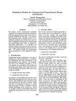
former. Strong LD was observed between closely linked
loci pairs (Fig. 2a). LD decayed to r2 =0.1 within 545 bp,
which corresponds approximately to a genetic map distance of 0.0008 cM. Based on the 10,000 simulated SNPs
distributed across the genome (Additional files 4 and 5),
the PCoA for the simulated parental inbreds revealed a
pattern of population structure similar to that of the original parental inbreds (Fig. 1b). LD decayed to r2 =0.1 within
0.08 cM (Fig. 2b).
For the scenario with 100 individuals in each of the
40 BC-NAM subpopulations, 50 QTLs, and h2 = 0.8,
the power of QTL detection 1 − β ∗ decreased with the
empirical α ∗ level decreasing from 0.5 to 0.00001 (Fig. 3,
Table 2, Additional files 6 and 7). The statistical power
of QTL detection 1-β ∗ of single marker model 1 and 2,
which did not include cofactors, was significantly lower
than that of JCIM model 1 and 2, which included the
selected cofactors. The statistical power of QTL detection 1-β ∗ of the models using cofactor selection method 2
was slightly higher than that for the models using cofactor
selection method 1. In case of a pure additively inherited
trait, the statistical power of QTL detection 1-β ∗ for the
models considering the marker or cofactor effects nested
within subpopulations (i.e. single marker model 1 and
JCIM model 1) was lower than that for the models considering marker or cofactor effects across subpopulations
(i.e. single marker model 2 and JCIM model 2). The power
trends were similar for other examined scenarios, irrespective of mating designs, sample sizes, QTL numbers,
and heritabilities. Moreover, for the difference between
the estimated QTL effects by the statistical models and

its relevant true (simulated) effects, the statistical model
which had higher power of QTL detection (for example,
JCIM model 2 with cofactor selection method 2) also had
a lower difference of QTL effect than those models with
lower power of QTL detection (Additional file 8).
However, the power of QTL detection 1-β ∗ for JCIM
model 1 was higher than that for JCIM model 2, when
examing a scenario in which a few (1–5) QTLs had additive effects as well as QTL × genetic background interaction effects with a few background markers ( 5) and with
a proportion of 50 % of the total variance explained by
the interaction (Fig. 4a, Additional file 9), or a scenario in
which there were interaction effects by many QTLs ( 25)
with more than 10 background markers and the proportion of the total variance explained by the interactions was
higher than 75 % (Fig. 4b, Additional file 10).


Li et al. BMC Plant Biology (2016) 16:26

Page 6 of 17

13

Panel 1
Panel 2
Common parent

0.15

b

0.20

a

0.10

4

0.05

28

11

18
14

3
2
45

42

34
32

7

1

22

26

49

19

6

27

35

5
36

−0.10 −0.05

48

12

8
17
21
20
9

0.00

PC 2 (2.3%)

15
16

29

46
47

10
40

39

30

43
41

33
44 37
51
50
23
24

31

25

38

−0.15

−0.10

−0.05

0.00

0.05

0.10

0.15

PC 1 (2.4%)

Fig. 1 Principal coordinate analysis of the 51 parental inbreds based on (a) the original 790 SNPs from 30 conserved genes and (b) the simulated
10,000 SNPs. PC 1 and PC 2 refer to the first and second principal coordinates, respectively. The numbers in parentheses refer to the proportion of
variance explained by the principal coordinates. Colors and symbols identify different sets of germplasm. The number 1–51 indicates the 51 of
parental inbreds, i.e. PBY001-004, PBY007, PBY010-015, PBY017-018, PBY021-027, PBY029, PBY031-041, PBY043-061, respectively (see Methods).
Number 51 is the common parental inbred used to simulate the nested association mapping populations

In a scenario in which the population sizes corresponded the sizes used in the Pre-BreedYield project
to create 21 DH-NAM and 29 BC-NAM subpopulations (with 100 individuals for each subpopulation) were
examined, the latter showed a significantly higher power
of QTL detection 1-β ∗ (e.g. 0.3785 at α ∗ = 0.01) than
the former (e.g. 0.2930 at α ∗ = 0.01). When the number
of involved parental inbreds and sample size was adjusted

to the same value for both mating designs, DH-NAM
and RIL-NAM mating designs showed a slightly (but not
significantly) higher power of QTL detection 1-β ∗ than
BC-NAM mating design (Fig. 5, Additional files 6, 7, 11,
12, 13, 14). The trends for the power of QTL detection
were similar, irrespective of QTL numbers, heritabilities,
the numbers of parental inbreds, and sample sizes. The
power of QTL detection 1-β ∗ decreased significantly


Li et al. BMC Plant Biology (2016) 16:26

Page 7 of 17

0.0

0.2

0.4

r2

0.6

0.8

1.0

a

00

200

300

400

500

600

Physical distance (bp)

b

Fig. 2 Nonlinear regression of the linkage disequilibrium measure r 2 against physical distance (bp) (a) based on the 790 original SNPs of the 51
parental inbreds and (b) based on 10,000 simulated SNPs of the simulated 51 parental inbreds. The red line is the nonlinear regression trend line of
r 2 vs. physical distance

when the number of simulated QTLs increased from 25
to 100 (Fig. 6, Additional files 15, 16, 17, 18). Further,
the power of QTL detection 1-β ∗ significantly increased
when the heritability was increased from 0.5 to 0.8. Similarly, the power of QTL detection 1-β ∗ increased when
the numbers of parental inbreds increased from 20 to 50
and the mapping population sizes increased from 2000 to
5000 (Fig. 7). With a constant total population size, the

mapping population consisted of 40 subpopulations with

50 individuals per subpopulation showed a slightly (but
not significantly) higher power of QTL detection 1-β ∗
than the mapping population consisted of 20 subpopulations with 100 individuals per subpopulation (Fig. 7). The
stronger the unbalancedness of the size of the individual
subpopulation was, the lower was the power of QTL
detection 1-β ∗ (Fig. 8).


Li et al. BMC Plant Biology (2016) 16:26

Page 8 of 17

Fig. 3 Power of QTL detection 1 − β ∗ of four statistical models combined with two cofactor selection methods at different α ∗ levels in a scenario
with 50 QTLs, heritability h2 = 0.8, and 40 backcross nested association mapping (BC-NAM) subpopulations which were randomly selected from a
total of 50 BC-NAM subpopulations. JCIM represents joint composite interval mapping. Colors indicate different statistical models. Vertical lines at
each point indicate the standard errors

The power of QTL detection 1-β ∗ decreased when the
proportion of the total genetic variance explained by QTL
× genetic background interactions was increased from
0 to 0.25, irrespective of the mating designs, QTL numbers, heritabilies, and mapping population sizes (Fig. 9,
Additional files 6, 7, 19, 20, 21).
A further comparison was performed for the power of
QTL detection 1-β ∗ between the JICIM model and JCIM
model using the same mapping data (i.e. 10 BC-NAM
subpopulations with 50 QTLs and heritability h2 = 0.8)
(Additional file 22). When the LOD value was set to 5.0 for
JICIM, the empirical α ∗ was close to 0.01 and the average
power of QTL detection 1-β ∗ was 0.052, which was much
lower than those for JCIM model 1 ad 2 (0.219 and 0.266,

respectively) at the same empirical α ∗ levels.

Discussions
Simulation of parental inbreds

Rapeseed is one of the most important oilseed crops in
the world. In order to efficiently select rapeseed varieties with improved yield and agronomic traits through
marker or genomics-based selection, mapping of elite
genes in diverse germplasm is required. This can be
achieved by applying appropriate statistical methods that
evaluate the association between genomic polymorphisms
and phenotypic variation in different types of mapping
populations [34].
Recently, the nested association mapping strategy was
suggested to combine the high power of QTL detection

from linkage analyses with the high mapping resolution
of association analysis [17]. The strategy is based on
RIL populations derived from crosses between a set of
parental inbreds and one common parent from a diverse
germplasm set. However, the evaluation of the NAM
strategy or other NAM-like strategies requires developing, genotyping, and phenotyping large RIL populations, which in turn requires large financial resources (cf.
[20]). Therefore, computer simulations are mandatory for
examining the properties and evaluating the performance
of the different described statistical models and methods.
We observed a total of 1605 SNPs from the sequences
of 30 conserved genes for the parental inbreds, with a
polymorphic rate of 11.19 %, which means about 1 SNPs
per 9.1 bp. The polymorphic rate found in our study was
considerably higher than that reported in prevous stuides [35, 36]. The difference might be explained by the

large number of inbreds (51 parental inbreds) and the
highly diverse germplasm (including exotic and adapted
germplasm) that was used for SNP detection in our study.
To check LD decay, we made a nonlinear regression of r2
versus the genetic map distance (cM) or physical distance
(bp) according to [27] and calculated the distance when
r2 =0.1. We observed that LD decayed on average within
545 bp to r2 =0.1. This number of bp corresponds roughly
to 0.0008 cM. The LD decay in our study was much faster
than in the studies of [37] and [38], where [37] found
that the expected r2 declined to the significance threshold (95th quantile of r2 for unlinked loci) within about 1


Li et al. BMC Plant Biology (2016) 16:26

Table 2 Summary of the nominal type I error rate α and power of QTL detection 1 − β ∗ of four statistical models combined with two cofactor selection methods (C1, C2) at different
α ∗ levels in a scenario with 50 QTLs, heritability h2 = 0.8, and 40 backcross nested association mapping (BC-NAM) subpopulations which were randomly selected from a total of 50
BC-NAM subpopulations, where α is the mean nominal type I error rate across the performed 25 simulation runs, α ∗ is the empirical type I error rate, S1 and S2 refer to single marker
model 1 and 2, J1 and J2 refer to joint composite interval mapping model 1 and 2. For details see ‘Methods’
α∗

S1

S2

J1C1

J2C1

J1C2

J2C2

α

1-β ∗

α

1-β ∗

α

1-β ∗

α

1-β ∗

α

1-β ∗

α

1-β ∗

0.00001

9.71 × 10−27

0.049

4.51 × 10−28

0.063

1.09 × 10−14

0.099

4.00 × 10−17

0.099

6.40 × 10−18

0.090

1.41 × 10−23

0.100

0.0001

9.68 × 10−26

0.052

5.69 × 10−28

0.064

5.01 × 10−14

0.102

3.99 × 10−16

0.105

5.35 × 10−17

0.096

1.41 × 10−22

0.101

0.001

6.06 × 10−19

0.100

1.54 × 10−21

0.113

5.05 × 10−11

0.188

2.86 × 10−13

0.190

3.87 × 10−12

0.177

3.31 × 10−16

0.184

0.01

6.41 × 10−11

0.238

2.50 × 10−12

0.248

5.17 × 10−5

0.398

1.68 × 10−5

0.433

3.23 × 10−5

0.391

5.25 × 10−6

0.417

0.05

1.33 × 10−6

0.405

3.84 × 10−7

0.429

1.00 × 10−2

0.600

8.13 × 10−3

0.660

1.20 × 10−2

0.620

8.79 × 10−3

0.695

0.1

8.12 × 10−5

0.506

3.53 × 10−5

0.544

4.22 × 10−2

0.696

3.86 × 10−2

0.747

4.94 × 10−2

0.706

4.51 × 10−2

0.768

0.5

1.34 × 10−1

0.830

1.17 × 10−1

0.844

4.42 × 10−1

0.908

4.37 × 10−1

0.920

4.57 × 10−1

0.896

4.54 × 10−1

0.917

Page 9 of 17

Li et al. BMC Plant Biology (2016) 16:26

Page 10 of 17

a

b

Fig. 4 Power of QTL detection 1-β ∗ of joint composite interval mapping (JCIM) model 1 (black line) and 2 (red line) with cofactor selection method
1 at different α ∗ levels in a scenario with heritability h2 = 0.8, 50 backcross nested association mapping (BC-NAM) subpopulations and (a) 0.5 of
explained ratio by QTL × genetic background interactions to the total genetic variance, where 1 QTL interacted with 5 background markers; (b) 0.75
of explained ratio by QTL × genetic background interactions to the total genetic variance, where each of 25 QTLs interacted with 10 background
markers. Vertical lines at each point indicate the standard errors

cM in a diverse germplasm set, and [38] found high levels of LD extending over about 2 cM in a set of 85 winter
oilseed rape types. The difference might be explained by
the following reasons. Firstly, different thresholds were
applied to measure LD decay. Secondly, in our study LD
decay within conserved genes was examined, whereas
the previous researches studied genome-wide LD decay

inferred from molecular markers. Thirdly, all studies were
done on different sets of germplasm.
Based on the global LD decay (within 1cM) in a large
and diverse rapeseed population, assuming a genome size
of at least 2,000 cM, and aiming at a coverage of at least
1 marker per cM, the research of [37] suggested that
considerably more than 2,000 markers would be required

Li et al. BMC Plant Biology (2016) 16:26

Page 11 of 17

Fig. 5 Power of QTL detection 1-β ∗ of joint composite interval mapping model 1 with cofactor selection method 1 for 40 double haploid nested
association mapping (DH-NAM) vs. 40 backcross nested association mapping (BC-NAM) vs. 40 nest association mapping based on recombinant
inbred lines (RIL-NAM) subpopulations at different α ∗ levels in a scenario with 50 QTLs and heritability h2 = 0.8. The 40 DH-NAM, BC-NAM or
RIL-NAM subpopulations were randomly selected from a total of 50 relevant DH-NAM, BC-NAM, or RIL-NAM subpopulations. Colors indicate the
DH-NAM, BC-NAM or RIL-NAM population. Vertical lines at each point indicate the standard errors

for genome-wide association studies. At the beginning of
our project, we only had the sequences of the 30 conservative genes. With the information from these sequences,
we could well examine the population structure of the
founder lines and know the allele frequencies among
the founder lines as well. This information provided the

basis for our computer simulations. Though 30 conserved
genes do not reflect the true genomic situation, however, it reflects better the genomic situation than ignoring
this information. Therefore, a total of 10 000 SNPs were
simulated based on the original SNPs from the conserved
genes. Such a simulated SNP set should have as similar

Fig. 6 Power of QTL detection 1-β ∗ of joint composite interval mapping model 1 with cofactor selection method 1 for different numbers of QTLs
(25, 50, 100) and different heritabilities (0.5, 0.8) at different α ∗ levels in a scenario of 29 backcross nested association mapping (BC-NAM)
subpopulations. Colors indicate combinations of different number of QTLs and heritabilities. Vertical lines at each point indicate the standard errors


Li et al. BMC Plant Biology (2016) 16:26

Page 12 of 17

Fig. 7 Power of QTL detection 1-β ∗ of joint composite interval mapping model 1 for different numbers of parental inbreds and backcross nested
association mapping (BC-NAM) subpopulations (indicated by different colors) at different α ∗ levels in a scenario with 50 QTLs and heritability h2 =
0.8. Vertical lines at each point indicate the standard errors

properties as possible as the original set with respect to
population structure and LD decay. We observed that our
simulated parental inbreds maintained allele frequencies,
and therewith also population structure, similar to the
original parental inbreds (Fig. 1b). The LD decay in the
simulated parental inbreds is about 100 times slower than
that in the original parental inbreds (Fig. 2b). Though we

could make more generations of random mating to get the
same LD decay as the original SNP set, this would require
considerable computational time and resources. This has
the potential to lead to a higher power of QTL detection
when using the simulated parent inbreds as the parents of
NAM population rather than the original parental inbreds
for all examined scenarios. However, the ranking for the

Fig. 8 Power of QTL detection 1-β ∗ of joint composite interval mapping model 1 with cofactor selection method 1 for varied sample sizes of
subpopulations with a standared deviation from 0 to 40 at different α ∗ levels in a scenario with 50 QTLs, heritability h2 = 0.8, and 50 backcross
nested association mapping (BC-NAM) subpopulations. Colors indicate different standard deviations for generating varied sample sizes of
subpopulations. Vertical lines at each point indicate the standard errors


Li et al. BMC Plant Biology (2016) 16:26

Page 13 of 17

Fig. 9 Power of QTL detection 1-β ∗ of joint composite interval mapping model 1 with cofactor selection method 1 for different explained ratio
(0, 0.05, 0.15, 0.25) by QTL × genetic background interactions to the total genetic variance at different α ∗ levels in a scenario with 50 QTLs,
heritability h2 = 0.8, and 40 backcross nested association mapping (BC-NAM) subpopulations. Colors indicate different explained ratio by QTL ×
genetic background interactions to the total genetic variance. Vertical lines at each point indicate the standard errors

power of QTL detection 1-β ∗ for the examined scenarios is expected not to change. Therefore we think that the
simulation of parental inbreds is a legitimate approach for
the questions to be examined in our study.
Comparison of power of QTL detection 1-β ∗ of the
examined statistical models for NAM

The single marker model was frequently used in the early
association mapping research. This model was used in
our study as a reference. We further introduced the JCIM
model in our study, where, similar to CIM, markers were
chosen as cofactors to control the genetic variation of
the genetic background. Considering the structure of the
NAM populations, we included a subpopulation effect in
all examined models.
As (1) the ranking of the examined statistical models with respect to the power of QTL detection 1-β ∗
was the same in all examined scenarios except the scenarios with QTL × genetic background interactions,
and (2) the BC-NAM mating design is important for
plant breeder to make use of the exotic germplasm
resouces, we discuss in the context of the comparison
of statistical methods for QTL detection only the results
of the scenario with 40 BC-NAM subpopulations (100
individuals per subpopulation), 50 QTLs, and heritability

h2 = 0.8.
We observed that the power of QTL detection 1-β ∗
for the JCIM model 1 and 2, which used cofactors, was
significantly higher than that of single marker model 1
and 2, which did not use cofactors (Fig. 3). However, the

former statistical models required much more computational effort to screen cofactors than the latter. The higher
power of QTL detection 1-β ∗ for the JCIM models than
the single marker models can be explained by the fact
that cofactors not only corrected for population stratification, but also for the genetic variation of other possibly
linked or unlinked QTL which led to an increasing QTL
detection power and better estimation of QTL effects [6].
Moreover, we observed a high power of QTL detection
1-β ∗ using cofactor 2 (selected by the method 2) and
smaller difference of QTL effects between the estimated
and true QTL effects than those using cofactor 1 (selected
by the method 1). This might be explained by the difference of the two cofactor selection methods. The method
1 detected only one marker from each examined segment
to be cofactor or not, whereas the method 2 used all markers for cofactor selection from the segments containing
cofactors previous identified by the method 1. Therefore,
more appropriate markers were used as cofactors from
each examined segment for the latter than the former.
However, the latter required much more computational
effort to screen cofactors than the former. Our results
indicate that the proposed cofactor selection method,
which was executed by LASSO function [39], was highly
efficient with regard to computation time even when dealing with a large number of variables. In the following we
only discuss the results of the JCIM models with cofactor
selection method 1.
We observed that the power of QTL detection 1-β ∗ for

the JCIM model 1 was significantly lower than that for the


Li et al. BMC Plant Biology (2016) 16:26

JCIM model 2 when the QTLs had only additive effects
(Fig. 3). This was also true when the QTLs had additive effects plus interaction effects with a low or medium
proportion of the total genetic variance explained by
many QTLs × genetic background interactions. The former model considered marker or cofactor effects nested
within subpopulations, whereas the latter model considered marker effects across subpopulations. This might be
because more parameters need to be estimated for the
former than the latter model, which in turn reduces the
power of QTL detection.
However, the power of QTL detection 1-β ∗ for JCIM
model 1 was higher than that for JCIM model 2 when
examing a scenario in which there were interaction effects
by a few (1–5) QTLs interacting with a few background
markers ( 5) (Fig. 4a) as well as a scenario in which
there were interaction effects by many QTLs ( 25) with
more than 10 background markers and the proportion of
the total variance explained by the interactions was higher
than 75 % (Fig. 4b).
In a NAM population, not all families have segregating
alleles at a given SNP locus, which might result in different
degrees of freedom of tested models and different levels
of probabilities for examined markers. However, this will
not affect the ranking of the examined statistical models
with respect to the power of QTL detection 1-β ∗ in our
study. The reasons are: (1) in our simulations, the power to
detect QTL at certain empirical type I error rates α ∗ were

compared. The power of QTL detection 1-β ∗ mainly relies
on the ranking of probabilities for non-QTL markers,
which will not be affected by the degree of freedom of the
tested models (for details see Methods); (2) furthermore,
when we compared the QTL detection power to detect
QTL for each scenario, we were based on the same segregating families, which had the same segregation alleles at
a given SNP locus.
In empirical studies where the extent of QTLs × genetic
background interactions is unknown, the JCIM model 2 is
suggested to be applied for a primary scan, as the model
in most cases showed a higher power of QTL detection
than JCIM model 1. Based on the results from the primary scan, a secondary scan is suggested to be applied
using the JCIM model 1 in a scenario in which there
were interaction effects by a few (1–5) QTLs interacting
with a few background markers ( 5) as well as a scenario in which there were complicated interaction effects
such as many QTLs (
25) with several background
markers.
Moreover, we observed that our proposed JCIM models
showed higher power of QTL detection than the existing
JICIM model (Additional file 22). The reason might be
due to that (1) our proposed cofactor selection methods
could effectively select cofactors to control the variation
of genetic bakcground during QTL mapping, and (2) our

Page 14 of 17

proposed models could effectively control the impact of
population structure. However, as the examined parameters and mapping procedures are different for these
models, a comprehensive comparison among the existing

statistical models for NAM analysis should be performed
in future.
Influence of mating designs on power of QTL detection

In the Pre-BreedYield project, two different sets of
germplasm, namely adapted and exotic germplasm, were
used. Accordingly, a DH-NAM mating design was applied
to the adapted germplasm because it required little time to
create fully homozygous genotypes via DH development
and thus make use of the elite germplasm resources. However, for the exotic germplasm, due to the likely reasons
of low compatibility, hybrid sterility, linkage drag, and
inferior performance of hybrids, it might require more
generations of backcrossing and selfing to overcome these
obstacles. In such cases, the BC-NAM mating design
might be appropriate when using exotic germplasm as
introgression donor parents. Therefore, the power of QTL
detection 1-β ∗ for the two mating designs were compared
in the study.
In a scenario of 40 DH-NAM vs. 40 BC-NAM subpopulations with 50 QTLs, heritability h2 = 0.8, and
100 individuals per subpopulation, we observed that the
DH-NAM mating design showed a slightly, but not significantly, higher power of QTL detection 1-β ∗ than the
BC-NAM mating design, irrespective of QTL numbers
and heritabilities examined (Fig. 5). This difference in
power estimates between the two mating designs might be
due to that the average allele frequencies for the DH-NAM
population were close to 0.5, whereas for the BC-NAM
design the common parental inbred had a higher allele frequency than the donor parental inbreds. This in turn leads
to a higher power of QTL detection for the DH-NAM
mating design than for the BC-NAM mating design. The
explanation could be supported by the findings of [19],

who observed that the differences in allele frequencies for
different crossing schemes contributed to the difference in
power estimates.
Influence of different genetic parameters on power of QTL
detection

In this study we examined the influence of (i) the genetic
architecture of the examined traits, (ii) the mapping
population size and the number of parental inbreds, and
(iii) unbalancedness of the size of the subpopulations on
the power of QTL detection 1-β ∗ .
Genetic architecture of the trait: We observed a higher
power of QTL detection 1-β ∗ for the traits assessed with
a high heritability than for the traits assessed with a low
heritability (Fig. 6). Similiar trends were observed for the
traits controlled by a low number of QTLs than for the


Li et al. BMC Plant Biology (2016) 16:26

traits controlled by a high number of QTLs. The reason is
that in the former case each QTL explained a higher proportion of the phenotypic variance than in the latter. For
the traits influenced by QTLs with both additive effects
and QTL × genetic background interaction, the power
of QTL detection was significantly lower than for those
influenced by QTLs with purely additive effects (Fig. 9).
Moreover, the higher the proportion of the total variance explained by QTL × genetic background interaction
was, the lower was the power of QTL detection 1-β ∗ .
Our observation was similar to the research of [40] and
could be explained by the fact that a high proportion of

the total variance by QTL × genetic background interaction reduced the proportion of the phenotypic variance
explained by each QTL, and thereby reduced the power of
QTL detection [18].
Mapping population size and the number of parental
inbreds: Across all examined scenarios, a higher power of
QTL detection 1-β ∗ was observed for the mapping populations with a higher number of individuals and parental
inbreds (Fig. 7). This observation was in accordance with
the results of [18] and could be explained by the fact that
in this case allele effects are estimated more precisely, and
that a higher number of parental inbreds increased the
number of polymorphic QTL [18]. Furthermore, with a
constant total population size, the mapping population
consisted of 40 subpopulations with 50 individuals per
subpopulation showed a slightly (but not significantly)
higher power of QTL detection 1-β ∗ than the mapping
population consisted of 20 subpopulations with 100 individuals per subpopulation (Fig. 7). The reason for this
might be that a higher number of subpopulations leads
to a higher number of parental inbreds and polymorphic
QTL in the total mapping population for the former than
the latter, and this in turn inceases the power of QTL
detection 1-β ∗ .
Unbalancedness of the size of the subpopulations: We
further examined the influcence of unbalancedness of the
size of the subpopulations on the power of QTL detection
1-β ∗ . Our results suggested that a mapping population
with an unbalanced size of the subpopulations had a significantly lower power of QTL detection 1-β ∗ than that
with a balanced size of the subpopulations, although the
total size of the mapping population was the same (Fig. 8).
The reason for this might be that an unbalanced size of
subpopulations leads to an unbalanced frequency of the

alleles of the individual parental inbred in the total mapping population, and this in turn has the potential to
reduce the power of QTL detection 1-β ∗ .
As no earlier studies reported results from nested association mapping in rapeseed, our research is indispensable to draw conclusions about the prospects of nested
association mapping in rapeseed. The results of our study
support the optimal design as well as analysis of NAM

Page 15 of 17

populations, especially in rapeseed. As nested association mapping can efficiently combine the advantages of
linkage mapping and association mapping, the developed
statistical models for NAM in this study is of importance
for detecting novel QTLs and preparing marker assisted
selection programs in rapeseed.

Conclusions
Our research showed that a joint composite interval mapping (JCIM) model had significantly higher power of QTL
detection than a single marker model. DH-NAM mating
design showed a slightly higher power of QTL detection than the BC-NAM mating design. The JCIM model
considering QTL effects nested within subpopulations
showed higher power of QTL detection than the JCIM
model considering QTL effects across subpopulations,
when examing a scenario in which there were interaction
effects by a few QTLs interacting with a few background
markers as well as a scenario in which there were interaction effects by many QTLs ( 25) each with more than
10 background markers and the proportion of total variance explained by the interactions was higher than 75 %,
vise versa. The results of our study support the optimal
design as well as analysis of NAM populations, especially
in rapeseed.

Availability of supporting data

The data sets supporting the results of this article
are included within the article and its additional files
(Additional files 1, 22, 8: see supplementary materials;
Additional files 2, 3, 4, 5, 6, 7, 9, 10, 11, 12, 13, 14, 15,
16, 17, 18, 19, 20, 21, i.e. Table S3 - Table S21, deposited
in the public repository Figshare with DOI: .
org/10.6084/m9.figshare.2009268).

Additional files
Additional file 1: Table S1. The information of the 30 conserved genes
and their annotations in Arabidopsis thaliana genome. Description: For
those having no gene annotation in A. thaliana genome, the start and end
positions in A. thaliana genome were given. (PDF 14.9 Kb)
Additional file 2: Table S20. Genotypes for the 51 parental inbreds at the
original SNPs. (TXT 186 kb)
Additional file 3: Table S21. A map file for the original SNPs. (TXT 31 kb)
Additional file 4: Table S3. Genotypes for the simulated 51 parental
inbreds at the simulated 10 K SNPs. (XLSX 31 kb)
Additional file 5: Table S4. Marker name and its position at chromosome
for the simulated 10 K SNPs. (XLSX 3133 kb)
Additional file 6: Table S5. Genotypes for the 50 BC-NAM
subpopulations, where 0 and 2 denote the homozygous gentoype of
parents, respectively, while 1 denotes the heterozygous genotype. (TXT
88,883 kb)
Additional file 7: Table S8. Phenotypes for the 50 BC-NAM
subpopulations in a scenario where QTLs = 50, h2 = 0.8 with 25
replications. (TXT 2088 kb)


Li et al. BMC Plant Biology (2016) 16:26

Additional file 8: Figure S1. Percentage of difference between estimated
and true (simulated) QTL effects for joint composite interval mapping
(JCIM) model 1 and 2 with cofactor selection method 1 and 2 in a scenario
with 50 QTLs, heritability h2 = 0.8, and 40 backcross nested association
mapping (BC-NAM) subpopulations. Description: Colors indicate different
statistical models and different cofactor sets. Vertical lines at each point
indicate the standard errors. (PDF 8.01 Kb)
Additional file 9: Table S9. Phenotypes for the 50 BC-NAM
subpopulations in a scenario where QTLs = 1 which interacted with 5
background markers, h2 = 0.8, 0.5 of explained ratio by QTL × genetic
background interactions to the total genetic variance with 25 replications.
(TXT 2078 kb)
Additional file 10: Table S10. Phenotypes for the 50 BC-NAM
subpopulations in a scenario where QTLs = 25, h2 = 0.8, 0.75 of explained
ratio by QTL × genetic background interactions to the total genetic
variance, each of 25 QTLs interacted with 10 background markers with 25
replications. (TXT 2078 kb)
Additional file 11: Table S6. Genotypes for the 50 DH-NAM
subpopulations, where 0 and 2 denote the homozygous gentoypes of
parents, respectively. (TXT 88,883 kb)
Additional file 12: Table S7. Genotypes for the 50 RIL-NAM
subpopulations, where 0 and 2 denote the homozygous gentoype of
parents, respectively, while 1 denotes the heterozygous genotype. (TXT
88,883 kb)
Additional file 13: Table S14. Phenotypes for the 50 DH-NAM
subpopulations in a scenario where QTLs = 50, h2 = 0.8 with 25
replications. (TXT 2088 kb)
Additional file 14: Table S15. Phenotypes for the 50 RIL-NAM
subpopulations in a scenario where QTLs = 50, h2 = 0.8 with 25

replications. (TXT 2078 kb)
Additional file 15: Table S16. Phenotypes for the 29 BC-NAM
subpopulations in a scenario where QTLs = 50, h2 = 0.5 with 25
replications. (TXT 1208 kb)
Additional file 16: Table S17. Phenotypes for the 29 BC-NAM
subpopulations in a scenario where QTLs = 25, h2 = 0.8 with 25
replications. (TXT 1208 kb)
Additional file 17: Table S18. Phenotypes for the 29 BC-NAM
subpopulations in a scenario where QTLs = 50, h2 = 0.5 with 25
replications. (TXT 1208 kb)
Additional file 18: Table S19. Phenotypes for the 29 BC-NAM
subpopulations in a scenario where QTLs = 100, h2 = 0.5 with 25
replications. (TXT 1208 kb)
Additional file 19: Table S11. Phenotypes for the 50 BC-NAM
subpopulations in a scenario where QTLs = 50, h2 = 0.8, 0.05 of explained
ratio by QTL × genetic background interactions to the total genetic
variance with 25 replications. (TXT 2078 kb)
Additional file 20: Table S12. Phenotypes for the 50 BC-NAM
subpopulations in a scenario where QTLs = 50, h2 = 0.8, 0.15 of explained
ratio by QTL × genetic background interactions to the total genetic
variance with 25 replications. (TXT 2088 kb)
Additional file 21: Table S113. Phenotypes for the 50 BC-NAM
subpopulations in a scenario where QTLs = 50, h2 = 0.8, 0.25 of explained
ratio by QTL × genetic background interactions to the total genetic
variance with 25 replications. (TXT 2088 kb)
Additional file 22: Table S2. Comparisions of the power of QTL
detection 1-β ∗ among the joint inclusive composite interval mapping
(JICIM) model, joint compositve interval mapping (JCIM) model 1 and 2.
Description: The comparisons were performed in a scenario with 50 QTLs,
heritability h2 = 0.8, cofactors selected by the Method 1, and 10 backcross

nested association mapping (BC-NAM) subpopulations which were
randomly selected from a total of 50 BC-NAM subpopulations. The
empirical type I error α ∗ was calculated based the mapping results from
JICIM model and the segregating markers and QTLs within the mapping
population. For details see Methods. (PDF 16.1 kb)

Page 16 of 17

Abbreviations
ANOVA: Analysis of variance; BC-NAM: Backcross nested association mapping;
CIM: Composite interval mapping; cM: centi Morgen; DH: Double haploid;
DH-NAM: Double haploid nested association mapping; ICIM: Inclusive
composite interval mapping; JCIM: Joint composite interval mapping; JICIM:
Joint inclusive composite interval mapping; LASSO: Least absolute shrinkage
and selection operator; LD: Linkage disequilibrium; LOD: Logarithm of odds;
MRD: Modified Rogers distance; NAM: Nested association mapping; PBY:
Pre-breed yield; PCoA: Principal coordinate analysis, QTL: Quantitative trait
locus; RIL: Recombinant inbred line; RIL-NAM: Recombinant inbred lines
nested association mapping; SSD: Single seed descent; SNP: Single nucleotide
polymorphism.
Competing interests
The authors declare that they have no conflict of interest.
Authors’ contributions
JL carried out the computer simulations, analyzed and interpreted the data,
drafted the manuscript. AB participated in analysis and interpretation of the
data, and revised the manuscript. VS provided and analyzed the sequence
data. BS conceived and supervised the study, interpreted the data, and revised
the manuscript. All authors read and approved the final manuscript.
Acknowledgements
The research was funded by the project “Precision breeding for yield gain in

Oilseed Rapes” which was supported by German Federal Ministry of Education
and Research and coordinated by Dr. Gunhild Leckband from German seed
alliance GmbH. The authors thank Prof. Dr. Maarten Koornneef, Director at Max
Planck institute for plant breeding research, Cologne and Dr. Fabio Fiorani
from the Forschungszentrum Jülich GmbH for their support during the
research, and thank the editor and the anonymous reviewers for their valuable
suggestions.
Author details
1 Max Planck Institute for Plant Breeding Research, Carl-von-Linné-Weg 10,
50829 Köln, Germany. 2 Syngenta Seeds GmbH, Zum Knipkenbach 20, 32107
Bad Salzuflen, Germany.
Received: 21 April 2015 Accepted: 7 January 2016

References
1. Kimber DS, McGregor DI. The Species and Their Origin, Cultivation and
World Production. Wallingford: CABI Publishing; 1995.
2. Becker HC, Engqvist GM, Karlsson B. Comparison of rapeseed cultivars
and resynthesized lines based on allozyme and rflp markers. Theor Appl
Genet. 1995;91:62–7.
3. Kebede B, Thiagarajah M, Zimmerli C, Rahman MH. Improvement of
open-pollinated spring rapeseed (Brassica napus l.) through introgression
of genetic diversity from winter rapeseed. Crop Sci. 2000;50:1236–43.
4. Falconer DS, Mackay TFC. Introduction to Quantitative Genetics, 4th edn.
London: Longman Group Ltd.; 1996.
5. Mackay TFC. The genetic architecture of quantitative traits. Annu Rev
Genet. 2001;35:303–39.
6. Zeng Z. Precision mapping of quantitative trait loci. Genetics. 1994;136:
1457–68.
7. Stich B, Melchinger AE. Comparison of mixed-model approaches for
association mapping in rapeseed, potato, sugar beet, maize, and

Arabidopsis. BMC Genomics. 2009;10:94.
8. Snowdon R, Luehs W, Friedt W. Oilseed Rape. Heidelberg: Springer; 2006.
9. Long Y, Shi J, Qiu D, Li R, Zhang C, Wang J, Hou J, et al. Flowering time
quantitative trait loci analysis of oilseed Brassica in multiple environments
and genome wide alignment with arabidopsis. Genetics. 2007;1777:
2433–44.
10. Thornsberry JM, Goodman MM, Doebley J, Kresovich S, Nielsen D,
Buckler ES. Dwarf8 polymorphisms associate with variation in flowering
time. Nat Genet. 2001;28:286–9.
11. Rafalski JA. Association genetics in crop improvement. Curr Opin Plant
Biol. 2010;13:1–7.
12. Wang N, Qian W, Suppanz I, Wei L, Mao B, Long Y, et al. Flowering time
variation in oilseed rape (Brassica napus L.) is associated with allelic


Li et al. BMC Plant Biology (2016) 16:26

13.

14.

15.

16.

17.

18.

19.

20.

21.

22.
23.

24.

25.

26.

27.

28.
29.
30.
31.
32.

33.
34.
35.

36.

variation in the FRIGIDA homologue BnaA.FRI.a. J Exp Bot. 2011;62:
5641–58.
Fritsche S, Wang X, Li J, Stich B, Kopisch-Obuch FJ, Endrigkeit J, et al. A

candidate gene-based association study of tocopherol content and
composition in rapeseed (Brassica napus). Frontiers in plant science.
2012;3:129.
Hasan M, Friedt W, Pons-Kühnemann J, Freitag N, Link K, Snowdon R.
Association of gene-linked ssr markers to seed glucosinolate content in
oilseed rape (Brassicanapus ssp. napus). Theor Appl Genet. 2008;116:
1035–49.
Honsdorf N, Becker HC, Ecke W. Association mapping for
phenological,morphological,and quality traits in canola quality winter
rapeseed (Brassica napus L.) Genome. 2010;53:899–907.
Zou J, Jiang CC, Cao ZY, Li RY, Long Y, Chen S, et al. Association mapping
of seed oil content in Brassica napus and comparison with quantitative
trai tloci identified from linkage mapping. Genome. 2010;53:908–16.
Yu J, Holland JB, McMullen MD, Buckler ES. Genetic design and statistical
power of nested association mapping in maize. Genetics. 2008;178:
539–51.
Stich B. Comparison of Mating Designs for Establishing Nested
Association Mapping Populations in Maize and Arabidopsis thaliana.
Genetics. 2009;183:1525–34.
Klasen J, Piepho H, Stich B. QTL detection power of multi-parental RIL
populations in Arabidopsis thaliana. Heredity. 2012;108(6):626–32.
Buckler ES, Holland JB, Bradbury PJ, Acharya CB, Brown PJ, Browne C,
et al. The genetic architecture of maize flowering time. Science. 2009;325:
714–8.
Soller M, Brody T, Genizi A. On the power of experimental design for
detection of linkage between marker loci and quantitative loci in crosses
between inbred lines. Theor Appl Genet. 1976;47:35–9.
Lander ES, Botstein D. Mapping mendelian factors underlying
quantitative traits using rflp linkage maps. Genetics. 1989;121:185–99.
Li HH, Bradbury P, Ersoz E, Buckler ES, Wang J. Joint qtl linkage mapping

for multiple-cross mating design sharing one common parent. Plos One.
2011;6:17573.
Bancroft I, Morgan C, Fraser F, Higgins J, Wells R, Clissold L, et al.
Dissecting the genome of the polyploid crop oilseed rape by
transcriptome sequencing. Nat Biotechnol. 2011;29(8):764–8.
Mangin B, Siberchicot A, Nicolars S, Doligez A, This P, Cierco-Ayrolles C.
Novel measures of linkage disequilibrium that correct the bias due to
population structure and relatedness. Heredity. 2012;108:285–91.
Ersoz ES, Yu J, Buckler ES. Application of linkage disequilibrium and
association mapping in maize. Berlin Heidelberg: Springer-Verlag; 2009,
pp. 173–195. Chap. 13.
Heuertz M, Emanuele DP, Källman T, Larsson H, Jurman I, Morgante M,
et al. Multilocus patterns of nucleotide diversity, linkage disequilibrium
and demographic history of Norway spruce (Picea abies (L.) Karst).
Genetics. 2006;174:2095–105.
Wright S. Evolution and Genetics of Populations, vol. IV. Chicago: The
University of Chicago Press; 1978.
Gower JC. Some distance properties of latent root and vector methods
used in multivariate analysis. Biometrika. 1966;53:325–38.
Lande R, Thompsont R. Efficiency of Marker-Assisted Selection in the
Improvement of Quantitative Traits. Genetics. 1990;124:743–56.
Efron B, Hastie T, Johnstone I. Least angel regression. Ann Stat.
2004;32(2):407–99.
Wang J, Li H, Zhang L, Li C, Meng L. Users Manual of QTL IciMapping,
V3.1 edn. Beijing, China: Institue of crop science, Chinese academy of
agricultural sciences; Crop research informatics lab, international maize
and wheat improvement center (CIMMYt); 2011.
R Development Core Team. R: A Language and Environment for Statistical
Computing. Vienna, Austria: R Foundation for Statistical Computing; 2011.
Doerge RW. Mapping and analyis of quantitative trait loci in experimental

populations. Nat Rev Genet. 2002;3:43–52.
Bus A, Hecht J, Huettel B, Reinhardt R, Stich B. High-throughput
popymorphism detection and genotyping in Brassica napus usning
next-generation rad sequencing. BMC Genomics. 2012;13:281.
Westermeier P, Wenzel G, Mohler V. Development and evalation of
single-nucleotide polymorphism markers in allotetraploid rapessed
(Brassica napus l.) Theor Appl Genet. 2009;119:1301–11.

Page 17 of 17

37. Bus A, Koerber N, Snowdon RJ, Stich B. Patterns of molecular variation in
a species-wide germplasm set of Brassica napus. Theor Appl Genet.
2011;123:1413–23.
38. Ecke W, Clemens R, Honsdorf N, Becker HC. Extent and structure of
linkage disequilibrium in canola quality winter rapessed (Brassica napus l.)
Theor Appl Genet. 2010;120:921–31.
39. Tibshirani R. Regression shrinkage and selection via the lasso. J R Stat Soc
Ser B. 1996;58:267–88.
40. Jannink JL. Identifying quantitative trait locus by genetic background
interactions in association studies. Genetics. 2007;176(1):553–61.

Submit your next manuscript to BioMed Central
and we will help you at every step:
• We accept pre-submission inquiries
• Our selector tool helps you to find the most relevant journal
• We provide round the clock customer support
• Convenient online submission
• Thorough peer review
• Inclusion in PubMed and all major indexing services
• Maximum visibility for your research

Submit your manuscript at
www.biomedcentral.com/submit