Pro SQL Server 2008 Analysis Services- P2

CHAPTER 2  CUBES, DIMENSIONS, AND MEASURES
31

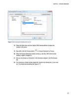
Figure 2-16. Selecting a different set of dimension members
To further analyze the results, we may drill into the date hierarchy to see how the numbers compare
by quarter or month. We could also compare these sales results to the sales of other products or number
of customers. Maybe we’d like to look at repeat customers in each area (is France outperforming Italy on
attracting new customers, bringing back existing customers, or both?). All these questions can be
answered by leveraging various aspects of this cube.
Incidentally, selection of various members is accomplished with a query language referred to as
Multidimensional Expressions, or more commonly MDX. You’ll be looking at MDX in depth in Chapter 9.
A question that may have come to mind by now: “Are measure values always added?” Although
measures are generally added together as they are aggregated, that is not always the case. If you had a
cube full of temperature data, you wouldn’t add the temperatures as you grouped readings. You would
want the minimum, maximum, average, or some other manner of aggregating the data. In a similar vein,
data consisting of maximum values may not be appropriate to average together, because the averages
would not be representative of the underlying data.
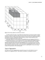
Types of Aggregation
OLAP offers several ways of aggregating the numerical measures in our cube. But first we want to
designate how to aggregate the data—either additive, nonadditive, or semiadditive measures.
Please purchase PDF Split-Merge on www.verypdf.com to remove this watermark.
CHAPTER 2  CUBES, DIMENSIONS, AND MEASURES
32
Additive
An additive measure can be aggregated along any dimension associated with the measure. When
working with our sales measure, the sales figures are added together whether we use the date dimension,
region, or product. Additive measures can be added or counted (and the counts can be added).
Semiadditive
A semiadditive measure can be aggregated along some dimensions but not others. The simplest example
is an inventory, which can be added across warehouses, districts, and even products. However, you can’t
add inventory across time; if I have 1,100 widgets in stock in September, and then (after selling 200

widgets) I have 900 widgets in October, that doesn’t mean I have 2,000 widgets (1,100 + 900).
Nonadditive
Finally, a nonadditive measure cannot be aggregated along any dimension. It must be calculated
independently for every set of data. A distinct count is an example of a nonadditive measure.

Note SQL Server Analysis Services has a semiadditive measure calculation named
AverageOfChildren
. You
might be confused about why this is considered semiadditive. It turns out that the way this aggregation operates is
that it sums along every dimension except a time dimension; along the time dimension, it averages (covering the
inventory example given earlier).
Writeback
Most of the time OLAP cubes are implemented, they are put in place as an analytic tool, so cubes are
read-only. On some occasions, users may want to write data back to the cube. We don’t want users
changing inventory or sales numbers from an analysis tool, so why would they want to change the
numbers?
A powerful analysis technique to offer your users is what-if or scenario analysis. Using this process,
analysts can change numbers in the cube to evaluate the longer-term effects of those changes. For
example, they might want to see what happens to year-end budget numbers if every department cuts its
budget by 10 percent. What happens to salaries? Capital expenses? Recurring costs? Although these
effects can be run with multiple spreadsheets, you could also create an additional dimension named
scenario, which analysts can use to edit data and view the outcomes. The method of committing those
edits is called writeback.
The biggest concern when implementing writeback on a cube is dealing with spreading. Consider
our time dimension (Figure 2-17). An analyst who is working on a report that shows calendar quarters
might want to change one value. When that value is changed, what do we do about the months? The
days?

Please purchase PDF Split-Merge on www.verypdf.com to remove this watermark.
CHAPTER 2  CUBES, DIMENSIONS, AND MEASURES

33

Figure 2-17. A calendar dimension
We have two choices. In our design, we can create a dimension that drills down to only the quarter
level. Then the calendar quarters are the leaf level of the dimension, the bottom-most level, and the
value for the quarter is just written into the cell for that quarter. Alternatively, some OLAP engines will
allow the DBA to configure a dimension for spreading; when the engine writes back to the cube, it
distributes the edited value to the child elements. The easiest (and usually default) option is to divide the
new value by the number of children and divide it equally. An alternative that may be available if the
analyst is editing a value is to distribute the new value proportionally to the old value.
Writeback in general, and spreading in particular, are both very processor- and memory-intensive
processes, so be judicious about when you implement them. You’ll look at writeback in Analysis Services
in Chapter 11.
Calculated Measures
Often you’ll need to calculate a value, either from values in the measure (for example, extended price
calculated by multiplying the unit cost by the number of items), or from underlying data, such as an
average.
Calculating averages is tricky; you can’t simply average the averages together. Consider the data in
Table 2-1, showing three classes and their average grades.
Table 2-1. Averaging Averages
Classroom Number of Students Average Score
Classroom A 20 100%
Classroom B 40 80%
Classroom C 80 75%

Please purchase PDF Split-Merge on www.verypdf.com to remove this watermark.
CHAPTER 2  CUBES, DIMENSIONS, AND MEASURES
34
You can’t simply add 100, 80, and 75 then divide by 3 to get an average of 85. You need to go back to
the original scores, sum them all together, and divide by the 140 students, giving an answer of 80

percent. This is another area where OLAP really pays off, because the OLAP engine is designed to run
these calculations as necessary, meaning that all the user has to worry about is selecting the analysis
they want to do instead of how it’s calculated.
Actions
Generally, an OLAP solution is the first-layer approach to analysis—it’s where you start. After you find
something of interest, you generally want additional information. One method of getting amplifying
data for something you find in an analysis is to drill through to the underlying data. Some analysis tools
provide a way of doing this directly, at least to the fact table; others don’t.
A more general way of gaining contextual insight into the data that you are looking at is to create a
structure called an action. This enables an end user to easily view amplifying data for a given dimension
member or measure. You can provide reports, drill-through data sets, web pages (Figure 2-18), or even
executable actions.


Figure 2-18. Using an action to open a map based on the member of the dimension
Actions are attached to objects in the cube—a specific dimension, hierarchy or hierarchy level,
measure, or a member of any of those. If the object will have several potential targets (as a dimension
has multiple members), you will have to set up a way to link the member to the target (parsing a URL,
creating a SQL script, passing a parameter to a report). For example, Listing 2-1 shows code used to
assemble a URL from the members selected in an action that opens a web-based map.
Please purchase PDF Split-Merge on www.verypdf.com to remove this watermark.
CHAPTER 2  CUBES, DIMENSIONS, AND MEASURES
35
Listing 2-1. Creating a URL from Dimension Members
// URL for linking to MSN Maps
" +

// Retreive the name of the current city
[Geography].[City].CurrentMember.Name + "," +

// Append state-province name
[Geography].[State-Province].CurrentMember.Name + "," +

// Append country name
[Geography].[Country].CurrentMember.Name +

// Append region parameter
"&regn1=" +

// Determine correct region parameter value
Case
When [Geography].[Country].CurrentMember Is
[Geography].[Country].&[Australia]
Then "3"
When [Geography].[Country].CurrentMember Is
[Geography].[Country].&[Canada]
Or
[Geography].[Country].CurrentMember Is
[Geography].[Country].&[United States]
Then "0"
Else "1"
End

This code will take the members of the hierarchy from the dimension member you select to
assemble the URL (the syntax is MDX, which you’ll take a quick look at in a few pages and dig into in
depth in Chapter 9). This URL is passed to the client that requested it, and the client will launch the URL
by using whatever mechanism is in place.
Other actions operate the same way: they assemble some kind of script or query based on the
members selected and then send it to the client. Actions that provide a drill-through will create a data set
of some form and pass that to the client.

All these connections are generally via XMLA.
XMLA
XML for Analysis (XMLA) was introduced by Microsoft in 2000 as a standard transport for querying OLAP
engines. In 2001, Microsoft and Hyperion joined together to form the XMLA Council to maintain the
standard. Today more than 25 companies follow the XMLA standard.
XMLA is a SOAP-based API (because it doesn’t necessarily travel over HTTP, it’s not a web service).
Fundamentally, XMLA consists of just two methods: discover and execute. All results are returned in
XML. Queries are sent via the execute method; the query language is not defined by the XMLA standard.
Please purchase PDF Split-Merge on www.verypdf.com to remove this watermark.
CHAPTER 2  CUBES, DIMENSIONS, AND MEASURES
36
That’s really all you need to know about XMLA. Just be aware of the transport mechanism and that
it’s nearly a universal standard. It’s not necessary to dig deeper unless you discover a need to.

Note For more information about XMLA, see
/>.
Multidimensional Expressions (MDX)
XMLA is the transport, so how do we express queries from OLAP engines? There were a number of query
syntaxes before Microsoft introduced MDX with OLAP Services in 1997. MDX is designed to work in
terms of measures, dimensions, and cubes, and returns structured data sets representing the
dimensional nature of the cube.
In working with OLAP solutions, you’ll work with both MDX queries and MDX statements. An MDX
query is a full query, designed to return a set of dimensional data. MDX statements are parts of an MDX
query, used for defining a set of dimensional data (for use in client tools, defining aspects of cube design,
and so forth).
A basic MDX query looks like this:

SELECT [measures] ON COLUMNS,
[dimension members] ON ROWS
FROM [cube]

WHERE [condition]

Listing 2-2 shows a more advanced query, and Figure 2-19 shows the results from a grid in Excel.
Listing 2-2. A More Advanced MDX Query
SELECT {DrilldownLevel({[Date].[Calendar Year].[All Periods]})} ON COLUMNS,
{DrilldownLevel({[Geography].[Geography].[All Geographies]})} ON ROWS
FROM
(
SELECT
{[Geography].[Geography].[Country].&[United States],
[Geography].[Geography].[Country].&[Germany],
[Geography].[Geography].[Country].&[France]} ON COLUMNS
FROM [Adventure Works]
)
WHERE ([Product].[Product Categories].[Category].&[1],[Measures].[Reseller Sales Amount])

Please purchase PDF Split-Merge on www.verypdf.com to remove this watermark.
CHAPTER 2  CUBES, DIMENSIONS, AND MEASURES
37

Figure 2-19. The results of the MDX query in Listing 2-2
When working with dimensional data, you can write MDX by hand or use a designer. There are
several client tools that enable you to create MDX data sets by using drag-and-drop, and then view the
resulting MDX. Just as with SQL queries, you will often find yourself using a client tool to get a query
close to what you’re looking for, then tweak it manually from the MDX.
Chapter 9 covers MDX in depth.
Data Warehouses
Data warehouse is a term that is loosely used to describe a unified repository of data for an organization.
Different people may use it to refer to a relational database or an OLAP dimensional data store (or both).
Conceptually, the idea is to have one large data “thing” that serves as a repository for all the

organization’s data for reporting and analytic needs.
The data warehouse may be a large relational data store that unifies data from various other systems
throughout the business, making it possible to run enterprise financial reports, perform analysis on
numbers across the company (perhaps payroll or absentee reports), and ensure that standardized
business rules are being applied uniformly. For example, when calculating absenteeism or consultant
utilization reports, are holidays counted as billable time? Do they count against the base number of
hours? There is no correct answer, but it is important that everyone use the same answer when doing the
calculations.
Many companies perform dimensional analysis against these large relational stores, just as you can
create a pivot table against a table of data in Excel. However, this neglects a significant amount of
research and investment that has been made into OLAP engines. It is not redundant to put a
dimensional solution on top of the relational store. Significant reporting can still be performed on the
relational store, leaving the cube for dimensional analysis. In addition, the data warehouse becomes a
staging database (more on those in a bit) for the cube. There are two possible approaches to building a
data warehouse: bottom-up or top-down.
Bottom-up design relies on departmental adoption of numerous small data marts to accomplish
analysis of their data. The benefit to this design approach is that business value is recognized more
quickly, because the data marts can be put into use as they come online. In addition, as more data marts
are created, business groups can blend in lessons learned from previous cubes. The downside to this
approach is the potential need for redesign in existing cubes as groups try to unite them later. The
software design analogy to bottom-up design is the agile methodology.
Top-down design attacks the large enterprise repository up front. A working group will put together
the necessary unifying design decisions to build the data warehouse in one fell swoop. On the plus side,
there is minimal duplication of effort as one large repository is built. Unfortunately, because of the
magnitude of the effort, there is significant risk of analysis paralysis and failure. Top-down design is
similar to software projects with big up-front or waterfall approaches.
Please purchase PDF Split-Merge on www.verypdf.com to remove this watermark.
CHAPTER 2  CUBES, DIMENSIONS, AND MEASURES
38
Data warehouses will always have to maintain a significant amount of data. So storage configuration

becomes a high-level concern.
Storage
Occasionally, you’ll have to deal with configuring storage for an OLAP solution. One issue that arises is
the amount of space that calculating every possibility can take. Consider a sales cube: 365 days; 1,500
products; 100 sales people; 50 sales districts. For that one year, the engine would have to calculate 365 ×
1,500 × 100 × 50 = 2,737,500,000 values. Each year. And we haven’t figured in the hierarchies (product
categories, months and quarters, and so forth).
Another issue here is that not every intersection is going to have a value; not every product is bought
in every district every day. The result is that OLAP is generally considered a sparse storage problem (for
every cell that could be calculated, most will be empty). This has implications both in designing storage
for the cube as well as optimizing design and queries for response time.
Staging Databases
When designing an OLAP solution, you will generally be drawing data from multiple data sources.
Although some engines have the capability to read directly from those data sources, you will often have
issues unifying the data in those underlying systems. For example, one system may index product data
by catalog number, another may do so by unique ID, and a third may use the nomenclature as a key.
And of course every system will have different nomenclature for red ten-speed bicycle.
If you have to clean data, either to get everyone on the same page or perhaps to deal with human
error in manually entered records (where is Missisippi?), you will generally start by aggregating the
records in a staging database. This is simply a relational store designed as the location where you unify
data from other systems before building a cube on top. The staging database generally will have a design
that is more cube-friendly than your average relational system—tables arranged in a more
fact/dimension manner instead of the normalized transactional mode of capturing individual records,
for example.

Note Moving data from one transactional system into another is best accomplished with an extract-transform-
load, or ETL, engine. SQL Server Integration Services is a great ETL engine that is part of SQL Server licensing.
Storage Modes
The next few sections cover storage of relational data; they are referring to caching data from the data
source, not this staging database. It’s possible to worry entirely too much about whether to use MOLAP,

ROLAP, or HOLAP—don’t. For 99 percent of your analysis solutions, your analysts will be using data
from last month, last quarter, or last year. They won’t be deeply concerned about keeping up with the
data as it changes, because it’s all committed and “put to bed.” As a result, MOLAP will be just fine in all
these cases.
ROLAP really becomes an issue only when you need continually updated data (for example, running
analysis on assembly line equipment for the current month). Although it’s important when it’s needed,
it’s generally not an issue. Let’s take a look at what each of these mean.
Please purchase PDF Split-Merge on www.verypdf.com to remove this watermark.
CHAPTER 2  CUBES, DIMENSIONS, AND MEASURES
39
MOLAP
Multidimensional OLAP (MOLAP) is probably what you’ve been thinking of to this point—the
underlying data is cached to the OLAP server, and the aggregations are precalculated and stored in the
OLAP server as well. This approach optimizes response time for queries, but because of the
precalculated aggregations, it does require a lot of storage space.
ROLAP
Relational OLAP (ROLAP) keeps the underlying data in the relational data system. In addition, the
aggregations are calculated and stored in the relational data system. The benefit of ROLAP is that
because it is linked directly to the underlying source data, there is no latency between changes in the
source data and the analytic results. Some OLAP systems may take advantage of server caching to speed
up response times, but in general the disadvantage of ROLAP aggregations is that because you’re not
leveraging the OLAP engine for precalculation and aggregation of results, analysis is much slower.
HOLAP
Hybrid OLAP (HOLAP) mixes MOLAP and ROLAP. Aggregations are stored in the OLAP storage, but the
source data is kept in the relational data store. Queries that depend on the preaggregated data will be as
responsive as MOLAP cubes, while queries that require reading the source data (aggregations that
haven’t been precalculated, or drilled down to the source data) will be slower, akin to the response times
of ROLAP.
We’ll review Analysis Services storage design in Chapter 12.
Summary

That’s our whirlwind tour of OLAP in general. Now that you have a rough grasp of what cubes are and
why we care about them, let’s take a look at the platform we’ll be using to build them—SQL Server
Analysis Services.
Please purchase PDF Split-Merge on www.verypdf.com to remove this watermark.
Please purchase PDF Split-Merge on www.verypdf.com to remove this watermark.
C H A P T E R 3

  

41
SQL Server Analysis Services
Now that you have a fundamental understanding of OLAP and multidimensional analysis, let’s start to
dig into the reason you bought this book: to find out how these OLAP technologies are implemented in
SQL Server, specifically SQL Server Analysis Services (SSAS). SSAS really came into its own in SQL Server
2005, which was a massive overhaul of the entire data platform from SQL Server 2000. SQL Server 2008
Analysis Services is more evolutionary than revolutionary, but still has significant improvements and
additions from the 2005 edition.
I wrote this chapter from the perspective of SSAS in the 2008 version (formerly code-named
Katmai). If you’re familiar with the 2005 version of SQL Server Analysis Services (formerly code-named
Yukon), you may just want to skip to the last section, where I call out the specific improvements in SQL
Server 2008 Analysis Services.
Requirements
Before I dive into the “all about SQL Server Analysis Services” stuff, you may want to install it. For a
detailed overview and instructions regarding installation of SQL Server 2008 and SSAS, see the SQL
Server 2008 Books Online topic “Initial Installation” at
library/bb500469.aspx. I’ll cover some of the high points here.
Hardware
I get a lot of questions about what kind of hardware to use for an Analysis Services installation. The
answer is, “It depends.” It depends on these factors:
• How many users you plan to support (and how quickly)

• What types of users you need to support (lightweight read-only reporting, or
heavy analysis?)
• How much data you have
• How fast you expect the data to grow
Generally, the hardware decision boils down to one of three scenarios:
New business intelligence initiative: Smallish amount of data, pilot group of users (fewer than ten).
Business intelligence initiative to satisfy large demand: For example, the current user base is using
Excel spreadsheets or an outdated software package against a fairly large existing body of data. So
Please purchase PDF Split-Merge on www.verypdf.com to remove this watermark.
CHAPTER 3  SQL SERVER ANALYSIS SERVICES
42
although there’s no current solution, you anticipate that when a solution is introduced, it will see
rapid adoption.
Replacing an existing solution: In this case, there is generally a large body of existing data that sees
heavy usage from a large number of users.

The first and third scenarios are the easiest to deal with. For the first scenario, you can start with a
single server and either install all the software on the physical machine or set up a virtual environment
reflecting a more mature architecture but on a single physical host (more on virtualization in a
moment). In the third scenario, you’ll have to do the hard-core analysis of the needs for data storage,
data growth, and usage. In other words, you know the answers—you just have to translate them.
The second scenario is the scary one. Your options seem to be either spend a ton of money on a
large-scale implementation, or run the possibility of setting up an architecture that your users outgrow
very quickly. The best approach here is to plan a small pilot and measured growth to a full
implementation, with provisions for scaling as necessary as usage and data storage needs grow.
Having said that, the minimum hardware requirements for SQL Server Analysis Services is a single-
core, single-CPU 1GHz CPU with 512MB RAM. Obviously, this is fairly silly; it’s almost impossible to buy
a server that doesn’t meet these specifications unless you’re shopping on eBay. My personal
recommendation for the hardware for a SQL Server Analysis Services implementation is as follows:
• Two dual-core CPUs. Multiple cores are great for multithreading, but the I/O

and cache architecture around discrete physical CPUs provide better
scalability. An alternative, should cost be an issue, would be to start with a
single dual-core CPU and plan to add a second when necessary. (Also be sure
to verify that your server will accept quad-core CPUs, and keep an eye on the
coming advances in eight-core CPUs and higher.)
• 4GB RAM, with capability to grow to 64GB. SSAS is an extremely memory-
hungry application.
• For the disk system, I’m partial to two drives in RAID 1 (mirrored) for the
system drive, and then a RAID 5 array for data. Some consider this fairly
complex for monitoring and management, so a single RAID 5 or RAID 10 array
can also serve. Analysis Services reads more than it writes, so read speed is far
more important that write speed.
ABOUT STORAGE-AREA NETWORKS
For large-scale storage, a lot of organizations immediately jump to storage-area networks, or SANs. A SAN
is an abstraction that allows creation of a large network-attached storage array. The SAN is maintained
and monitored by itself, and then various servers can attach to the SAN; they see it as a logical virtual drive
(called a LUN).
The benefit of a SAN is that it’s a single drive array that can be maintained with much closer attention
than, say, arrays scattered across a large number of servers in a data center. The downside of a SAN is
that it’s expensive, complicated, and a single point of failure. In addition, for a lot of enterprise-class
software, there needs to be a special infrastructure for supporting the software on a SAN.
Please purchase PDF Split-Merge on www.verypdf.com to remove this watermark.
CHAPTER 3  SQL SERVER ANALYSIS SERVICES
43
Depending on your anticipated architecture, needs, and whether your organization already has a SAN, you
might be better served by simply leveraging RAID arrays in servers and ensuring that you have capable
monitoring software. Most important (whether you have a SAN or not) is, of course, that you have the
processes in place to deal with hardware failures.
Virtualization
I mentioned virtualization earlier. Virtualization was made popular by VMware over the last ten years,

and Microsoft now offers both Virtual Server for Windows Server 2003, and Hyper-V technologies on
Windows Server 2008. I’m not sure that virtualization is a good idea with SSAS in the grand scheme of
things. It’s such a resource-intensive service that you’ll generally lose more than you gain. The only time
I would advocate it is if you’re just starting out; you could set up a virtualized network on a single server,
and then move virtual machines to physical machines as necessary (see Figure 3-1).


Figure 3-1. Scaling up from virtual to physical
In Figure 3-1, the solution was originally set up as five virtual servers on a single physical box. As the
solution grew, the first place we started seeing limitations were on the SSAS box (RAM) and the OLAP
relational store (hard drive space and I/O speed). So in a planned migration, we back up each server and
restore it to a new physical server to give us the necessary growth and headroom.
Please purchase PDF Split-Merge on www.verypdf.com to remove this watermark.
CHAPTER 3  SQL SERVER ANALYSIS SERVICES
44

Note The Microsoft support policy for virtualization can be found at
www.microsoft.com/sqlserver/
2008/en/us/virtualization.aspx
. The basic support policy is that SQL Server 2008 is supported on Hyper-V
guests. However, for other virtualization solutions (for example, VMware), Microsoft’s support is best effort (if
something can be resolved in the virtual environment, Microsoft will do its best to assist). However, if at any time it
becomes possible that the problem is related to the virtualization environment, you’ll be required to reproduce the
problem directly on hardware.
Software
To answer the first question in the realm of the 2008 Servers: No, you can’t install SQL Server 2008 on
Windows Server 2008 Core. You can install it on Windows Server 2003 SP2 or later, or Windows Server
2008. SQL Server Standard Edition can also be run on Windows XP SP2 or Vista. SQL Server x86 (32-bit)
can be run on either x86 or x64 platforms, while x64 (64-bit) can run only on x64 platforms.


Tip Although SQL Server 2008 is supported on a domain controller, installing it on one is not recommended.
SQL Server setup requires Microsoft Windows Installer 4.5 or later (you can be sure that the latest
installer is installed by running Windows Update). The SQL Server installer will install the software
requirements if they’re not present, including the .NET Framework 3.5 SP1, the SQL Server Native Client,
and the setup support files. Internet Explorer 6 SP1 or later is required if you’re going to install the
Microsoft Management Console, Management Studio, Business Intelligence Development Studio, or
HTML Help.

Note Installation of Windows Installer and the .NET Framework each require rebooting the server, so plan
accordingly.
Upgrading
Upgrading from SQL Server 2000 to 2005 was a fairly traumatic experience, because of the massive
architecture changes in the engine, storage, and features. Although some features have been deprecated
or removed in SQL Server 2008 as compared to 2005, the migration is far smoother.
The bottom line with respect to upgrading: If you have SQL Server 2005 installations that you have
upgraded from SQL Server 7 or 2000, the migration to 2008 should be much easier. More important, if
you have current SQL Server 2000 installations and you are evaluating migration to SQL Server 2005, you
should move directly to SQL Server 2008.
Consider one more point when evaluating upgrading from SQL Server 2005 to 2008. A number of my
customers have only recently finished upgrading to SQL Server 2005 and are understandably concerned
Please purchase PDF Split-Merge on www.verypdf.com to remove this watermark.
CHAPTER 3  SQL SERVER ANALYSIS SERVICES
45
about another migration effort so soon. There is no reason your server farm has to be homogeneous—
for example, you could upgrade your Analysis Services server to 2008 while leaving the relational store at
2005. Evaluate each server role independently for upgrade, because each role offers different benefits to
weigh against the costs.
Resources for upgrading to SQL Server 2008 can be found at
library/cc936623.aspx, including a link to the Upgrade Technical Reference Guide.
Standard or Enterprise Edition?

When you decide to go with SQL Server 2008 Analysis Services, a big decision to make is whether to go
with Standard or Enterprise Edition. In general, Standard Edition is for smaller responsibilities, and
Enterprise Edition is for larger, more mission-critical jobs. One easy way to differentiate is to ask
yourself, “Can I afford for this server to go down?” If not, you probably want to look at Enterprise Edition.

Note The full comparison chart for SQL Server’s Standard and Enterprise Editions is at
www.microsoft.com/
sqlserver/2008/en/us/editions.aspx
.
With SQL Server 2000, the primary differentiator was that you could cluster Enterprise Edition while
you couldn’t cluster Standard Edition. That alone was pretty much the deal-maker for most people. In
SQL Server 2005, you could cluster Standard Edition to two nodes, which seemed to remove a lot of the
value of Enterprise Edition (not quite true—there are still a lot of reasons to choose Enterprise Edition).
SQL Server 2008 adds a lot of features, and a majority of them are only in the Enterprise Edition.
From an Analysis Services perspective, features that are available only in Enterprise Edition include the
following:
Scalable shared databases: In SQL Server 2005, you could detach a read-only database and park it
on a shared cluster for use as a reporting database. In SQL Server 2008, you can do this with a cube
after the cube is calculated. You detach the cube and move it to central storage for a farm of front-
end database servers. Users can then access this farm by using tools such as Excel, ProClarity, or
PerformancePoint for analysis and reporting.
Account intelligence: This feature enables you to add financial information to a dimension that
specifies account data and then sets the dimension properties to be appropriate to that account
type. For example a “statistical” account type would have no aggregation, whereas an “asset”
account type would be set to aggregate the last nonempty member (similar to an inventory
calculation).
Linked measures and dimensions: I’ve explained that instead of having one large cube, you often
want to create several smaller cubes. However, you may have shared business logic or dimensions
(who wants to create and maintain the corporate structure dimension over and over?). Instead, you
can create a linked measure or linked dimension, which can be used in multiple cubes but

maintained in one location.
Semiadditive measures: As I mentioned in Chapter 2, you won’t always want to aggregate measures
across every dimension. For example, inventory levels shouldn’t be added across a time dimension.
Semiadditive measures provide the ability to have a measure aggregate values normally in several
directions, but then perform a different action along the time dimension.
Please purchase PDF Split-Merge on www.verypdf.com to remove this watermark.
CHAPTER 3  SQL SERVER ANALYSIS SERVICES
46
Perspectives: When considering cubes for large organizations, the number of dimensions,
measures, and members can get pretty significant. The AdventureWorks demo cube has 21
dimensions and 51 measures, and it’s focused on sales. Browsing through dozens or hundreds of
members can get old if you have to do it frequently. Perspectives offer a way of creating “views” on a
cube so that users in specific roles get shorter, focused lists of dimensions, measures, and members
suiting their role.
Writeback dimensions: In addition to being able to write back to measures, it’s possible to enable
your users to edit dimensions from a client application (as opposed to working with the dimension
in BIDS). Note that dimension writeback is possible only on star schemas.
Partitioned cubes: Also mentioned in Chapter 2, the ability to partition cubes makes maintenance
and scaling of large cubes much, much easier. When you can shear off the last 12 years of sales data
into a cube that has to be recompiled on only rare occasions, you do a lot for the ability to rebuild
the current cube more often.
Architecture
SQL Server Analysis Services runs as a single service (msmdsrv.exe) on the server. The service has several
components, including storage management, a query engine, XMLA listener, and security processes. All
communication with the service is via either TCP (port 2383) or HTTP.
The Unified Dimensional Model
A major underlying concept in Analysis Services is the unified dimensional model, or UDM. If you
examine more-formal business intelligence, data modeling, or OLAP literature, you will often find
something similar to Figure 3-2. Note the requirement for a staging database (for scrubbing the data), a
data warehouse (for aggregating the normalized data), data marts (for severing the data into more-

manageable chunks), and finally our OLAP store. I have seen architecture with even more data
redundancy!

Please purchase PDF Split-Merge on www.verypdf.com to remove this watermark.
CHAPTER 3  SQL SERVER ANALYSIS SERVICES
47

Figure 3-2. A traditional BI architecture
Apart from the duplication of data (requiring large amounts of disk space and processing power to
move the data around), we also have the increased opportunity for mistakes to surface in each data
translation. But the real problem we face is that systems like these often seem to end up like Figure 3-3.
Various emergent and exigent circumstances will create pockets and pools of data, and cross
connections, and it will all be a mess.


Figure 3-3. Does this look familiar?
Please purchase PDF Split-Merge on www.verypdf.com to remove this watermark.
CHAPTER 3  SQL SERVER ANALYSIS SERVICES
48
SSAS is designed to conceptually unify as much of Figure 3-2 as possible into a single-dimensional
model, and as a result make an OLAP solution easier to create and maintain. Part of what makes this
possible is the data source view (DSV), which is covered in Chapter 5. The DSV makes it possible to
create a “virtual view,” collating tables from numerous data sources. Using a DSV, a developer can create
multiple cubes to address the various business scenarios necessary in a business intelligence solution.
The net result is Figure 3-4—less data redundancy and a more organized architecture.


Figure 3-4. How Analysis Services enables the unified dimensional model
As I’ve mentioned previously, in many cases the data in the source systems isn’t clean enough for
direct consumption by a business intelligence (BI) solution. In that case, you will need a staging

database, which is designed to be an intermediary between the SSAS data source view(s) and the source
systems. This is similar to Figure 3-5, which also shows various clients consuming the cube data.

Please purchase PDF Split-Merge on www.verypdf.com to remove this watermark.
CHAPTER 3  SQL SERVER ANALYSIS SERVICES
49

Figure 3-5. Using a staging database to clean data before the SSAS server
There is still a lot of potential for complexity. But I hope you see that by using one or more data
source views to act as a virtual materialized view system, combined with the power of cubes (and
perspectives, as you’ll learn later), you can “clean up” a business intelligence architecture to make
design and maintenance much easier in the long run.
Logical Architecture
Figure 3-6 shows the logical architecture of Analysis Services. A single server can run multiple instances
of Analysis Services, just as it can run several instances of the SQL Server relational engine. (You connect
to an Analysis Services instance by using the same syntax: [server name] \ [instance name].) Within
each instance is a server object that acts as the container for the objects within.
Each server object can have multiple database objects. A database object consists of all the objects
you see in an Analysis Services solution in BIDS (more on that later). The minimum set of objects you
need in a database object is a dimension, a measure group, and a partition (forming a cube).

Please purchase PDF Split-Merge on www.verypdf.com to remove this watermark.
CHAPTER 3  SQL SERVER ANALYSIS SERVICES
50

Figure 3-6. SQL Server Analysis Services logical architecture
I’ve grouped the objects in a database into three rough groups:
OLAP objects: Consisting of cubes, data sources, data source views, and dimensions, these are the
fundamental objects that we use to build an OLAP solution. This is an interesting place to consider
the object model as it relates to our OLAP world (Figure 3-7).

Please purchase PDF Split-Merge on www.verypdf.com to remove this watermark.