Logic kỹ thuật số thử nghiệm và mô phỏng P4

165

Digital Logic Testing and Simulation

,

Second Edition

, by Alexander Miczo
ISBN 0-471-43995-9 Copyright © 2003 John Wiley & Sons, Inc.

CHAPTER 4

Automatic Test Pattern Generation

4.1 INTRODUCTION

In Chapter 3 we looked at fault simulation. Its purpose is to evaluate test programs in
order to measure their effectiveness at distinguishing between faulty and fault-free
circuits. The question of the origin of test stimuli was ignored for the moment; we
simply noted that test programs could be derived from test stimuli originally
intended for design verification, or stimuli could be written specifically for the pur-
pose of exercising the circuit to reveal the presence of physical defects, or stimuli
could be produced by an automatic test pattern generator (ATPG). We now turn our
attention to the ATPG. However, we also examine two alternatives to fault simula-
tion in this chapter: testdetect and critical path tracing. These two methods share
much common terminology, as well as methodology, with corresponding ATPGs, so
it is convenient to group them with their corresponding ATPGs.
A number of techniques have emerged over the past three decades to generate test
programs for digital circuits. For combinational circuits several of these, including
D-algorithm, PODEM, FAN and Boolean differences, have been shown to be true

algorithms, in the sense that, given enough time, they will eventually come to a halt;
that is, there is a stopping rule. If one or more tests exist for a given fault, they will
identify the test(s). For sequential circuits, as we will see in the next chapter, no such
statement can be made. Push-button solutions capable of automatically generating
comprehensive test programs for sequential circuits require assistance in the form of
design-for-test (DFT), which will be a subject for a later chapter. In this chapter, we
will examine the algorithms and procedures for combinational logic and attempt to
understand their strengths and weaknesses.

4.2 THE SENSITIZED PATH

In Section 3.4, while discussing the stuck-at fault model, it was pointed out that
whenever fault modeling alternatives were considered, combinatorial explosion

166

AUTOMATIC TEST PATTERN GENERATION

resulted. The number of choices to make, or the number of problems to solve, liter-
ally explodes. The stuck-at fault model is a necessary consequence of the combina-
torial explosion problem. A further consequence of this problem is the

single-fault
assumption

. When attempting to create a test, it is assumed that a single fault exists.
Experience with the stuck-at fault model and the single-fault assumption indicates
that they are effective; that is, a good stuck-at test that detects all or nearly all single
stuck-at faults in a circuit will also detect all or nearly all multiple stuck-at faults and
short faults.

The stuck-at fault has been defined as the fault model of interest for basic logic
gates, and tests for detecting stuck-at faults on these gates have been defined. How-
ever, individual logic gates do not occur in practice. Rather, they are interconnected
with many thousands of other similar gates to form complex circuits. When embed-
ded in a much larger circuit, there is no immediate access to the gate. Hence it
becomes necessary to use surrounding circuitry to set up the inputs to the gate under
test and to cause the effects of the fault to travel forward and become visible at an
output pin where these effects can be observed by a tester.

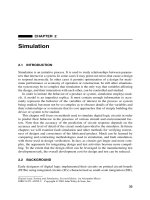
4.2.1 The Sensitized Path: An Example

The circuit in Figure 2.43, repeated here as Figure 4.1, will be used to illustrate the
process. The goal is to find a test for an SA0 on input 3 of gate

K

(i.e., the input
driven by gate

H

; on schematic drawings, inputs will be numbered from top to bot-
tom). Since gate

K

is an OR gate, the test for input 3 SA0 requires that input 3 be set
to 1 and the other inputs be set to 0. Two problems must be solved: First, logic
values must be computed on the primary inputs that cause the assigned test values to
appear at the inputs of

K

. Second, the values assigned to the primary inputs must
make the fault effect visible at the output. In addition, the values computed on the
primary inputs during these operations must not conflict.

Figure 4.1

Sensitizing a path.
I
1
I
2
I
3
I
4
I
5
Z
A
F
G
H
J
B
C
D
E

L
K
N
O
PM

THE SENSITIZED PATH

167

We attempt to create a sensitized path from the fault origin to the output. A

sensi-
tized path

of a fault

f

is a signal path originating at the fault origin

f

whose value all
along the path is functionally dependent on the presence or absence of the fault. If the
sensitized path terminates at a net that is observable by test equipment, then the fault is

detectable

. From the response at the output, it can be determined whether or not the tar-

geted fault occurred. The process of extending a sensitized path is called

propagation

.
Gate

H

, which drives the faulted input of gate

K

, is an AND gate, and a logic 1 on
its output only occurs if all its inputs have logic 1 values. This is called

implication

; a
1 on the output of an AND gate implies logic 1 on all its inputs. This implication oper-
ation can be taken a step further. The top input of H is driven directly by

I

2

, and its
bottom input is driven by

I

1

. Hence, both of these inputs must be assigned a logic 1.
This implication operation can be applied yet again. A 1 on the input to inverter

A

implies a 0 on its output, and that 0 drives gate

G

. Therefore, the output of gate

G

is a
0. Fortunately, that 0 is consistent with the initial values assigned to the inputs of

K

.
Other implications remain.

I

2

drives NOR gate

F

with a 1, causing the output of gate

F

to become 0. Again, that value is consistent with the original assignments to

K

.
Finally,

I

1

drives NOR gate

J

, and gate

J

responds with a 0, so once again the assign-
ment is consistent with the required values on

K

.
All that remains to get a 1 from gate

H

is to get 1s from gate

B

and gate

C

. Gate

B

is a two-input NAND gate, and it generates a 1 if either of its inputs is a 0. We
choose

I

3

and set it to 0. We still need to get a 1 from gate

C

. It is a two-input OR
gate and its upper input, from

I

3

, was already set to 0. So, we set

I

4

to 1.
All of the inputs to

K

have now been satisfied, so the output of

K

is a 0 if the
NOR gate is operating correctly, and the output of

K

is 1 if the fault exists. At this
point we introduce the D-notation. The letter D (discrepancy) represents a

composite
signal

1/0, where the first number represents the value on the fault-free circuit, and
the second number represents the value on the faulty circuit. The letter D represents
the composite signal 0/1, meaning that the fault-free circuit has the value 0 and the
faulty circuit has the value 1. The output of gate

K

is D.
A D will now be propagated forward through gate

M

. To do so requires a logic 1
on the other input to

M

, driven by gate

L

. The output of gate

D

is a 0, by virtue of the
0 on input

I

3

. However, a 1 can be obtained from gate

E

by assigning a 1 to input

I

5

.
All of the inputs have now been assigned; the values are

I

1

,

I

2

,

I

3

,

I

4

,

I

5

= (1,1,0,1,1).
However, a problem seems to appear. NAND Gate

M

has a D and a 1 on its
inputs. That produces a D on the output. Now, gate

N

has a D and a D on its inputs.
That means that the fault-free circuit applies 0 and 1 to gate

N

, and the faulty cir-

cuit applies 1 and 0. So both the fault-free and the faulty circuits respond with a 0
on the output of gate

N

. One solution is to back up to the last assignment,

I

5

= 1,
and change it to

I

5

= 0, so that the assignments on the primary inputs are

I

1

,

I

2

,

I

3

,

I

4

,

I

5

= (1,1,0,1,0). Then, the output of

E

becomes 0. That causes the output of

L

to
become 0, which in turn causes the output of

M

to become 1. A D
and 1 on the
input to

N

cause a D to appear on its output. Since

L

= 0, the other input to

P

is 0,
and the D makes it through

P

to the output

Z. As we will see, if we had considered
all possible propagation paths, this last operation, changing the value on I
5
, would
not have been necessary.
168
AUTOMATIC TEST PATTERN GENERATION
4.2.2 Analysis of the Sensitized Path Method

The operation that just took place will now be analyzed, and some observations will
be made. The process of backing up and changing assignments is called justifica-
tion, also sometimes referred to as the consistency operation. The two processes,
propagation and justification, can be used to find a test for almost any fault in the cir-
cuit (redundant logic, as we shall eventually see, presents testing problems). Fur-
thermore, propagation and justification can be applied in either order. We chose to
start by propagating from the point of fault to an output. It would be possible to first
justify the assignments on the four inputs of gate H, then propagate forward to the
output, one gate at a time, each time justifying all assignments made in that step of
the propagation.
During the propagation phase all required assignments are placed on the assign-
ment stack. Then, in the justification phase, the assignment stack expands and con-
tracts. When the stack is finally empty, the justification phase is complete. In the
second approach, processing begins with the justification process, attempting to sat-
isfy initial assignments on the gate whose input or output is being tested. Each time
the assignment stack empties, control reverts to the propagation mode and the sensi-
tized path extends one gate closer to the outputs. Then, control again reverts to the
justification routine until the assignment table is again empty. Control passes back
and forth in this fashion until the sensitized path reaches an output and all assign-
ments are satisfied.
Implication When assignments are made to individual gates, they sometimes
carry implications beyond the immediate assignment. An implication is an assign-
ment that is a direct consequence of another assignment. Only one assignment is
possible. Consider the assignment of a logic 1 to the output of gate H. This implied
that all of its inputs must be 1, implying that I
1
and I
2
must both be 1. Once I
1

had
been assigned a 1, that implied a 0 on the output of inverter A, which in turn implied
a 0 on the output of G. These operations will be stated more formally in a later sec-
tion, because now it is sufficient to point out that these implications obviated the
need to make choices at various points during the operation.
The Decision Table During propagation and justification, gates are encountered
where choices must be made. For example, when a 0 was required from the NOR
gate labeled F, the value 1 was assigned to the upper input. This choice caused a
problem because it resulted in an assignment I
1
= 0 that conflicted with a previous
assignment I
1
= 1. Because a choice existed, it was possible to back up and make an
alternate choice that eventually proved successful. In large, complex circuits with
much fanout, complex multilevel decisions often must be made. If all decisions at a
given gate have been tried without success, then the decision stack must be popped
and a decision made at the next available decision point. Furthermore, assignments
to all gates following the point at which the decision was made must be erased, and
any mechanism used to keep track of decisions for the gate that was popped off the
decision stack must be reset. The decision table maintains a record of choices, or
alternatives.
THE SENSITIZED PATH
169
The implication operation is of value here because it can often eliminate a num-
ber of decisions. For example, the initial test for gate H assigned a logic 1 to input I
2
.
But assigning a 1 to I
2

forces—that is, implies—a 0 on the output of gate F. As a
result, if implication is performed, there is no need to justify F = 0, and that in turn
eliminates the need to make a decision at gate F.
The Fault List The fault, input 3 of gate K, was selected arbitrarily in order to
demonstrate propagation and justification techniques. In actual practice the entire set
of stuck-at faults would be compiled into a fault list. That list would then be col-
lapsed using dominance and equivalence (cf. Section 3.4.5). Each time a test vector
is created for a fault in the circuit, that test vector would be fault simulated in order
to determine if any other faults are detected. The objective is to avoid performing
test vector generation on faults that have already been detected.
For example, the test for input 3 of K SA1 causes the fault-free circuit to assume
the value Z = 0. If input 3 of K were actually SA1, the output would assume the
value 1. But several other faults would also cause Z to assume the value 1, the most
obvious being the output of P SA1. Other faults causing a 1 output include outputs
of gate N or gate O SA1. In fact, any fault along the sensitized path that causes the
value on that path to assume a value other than the correct value will be detected by
the test vector.
The importance of this observation lies in the fact that if we can determine
which previously undetected faults are detected by each new test vector, then we
can check them off in the fault list and do not need to develop test vectors to spe-
cifically test for these faults. Several techniques for accomplishing this will be
described later.
Making Choices The sensitized path method for generating tests was used
during the early 1960s.
1
When this method reached a net with fanout during propa-
gation, it arbitrarily selected a single path and continued to pursue its objective of
reaching an output. Unfortunately, this blind pursuit of an output occasionally
ignored easy solutions.
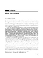
Consider what happens when an attempt is made to propagate a test through gate

M in Figure 4.2. Assume that the inputs to gates M and Q are primary inputs and that
the upper input to gate N is driven by other complex logic. Assume also that gate P
drives a primary output while gate N drives other complex logic. Gate P is not diffi-
cult to control. Its lower input, driven by gate Q, can be set to 1 with a 0 at either
input to Q. Gate N represents greater difficulties because a logic assignment at its
upper input must be justified through other logic, and a test at its output must be
propagated through additional logic. An arbitrary propagation choice could result in
an attempt to drive a test through the upper gate. In fact, if a program did not
examine the function associated with the fanout to gate P, it might go right past a
primary output and attempt to propagate a test through complex sequential logic at
the output of gate N.
170
AUTOMATIC TEST PATTERN GENERATION
Figure 4.2 Choosing the best path.
By ordering the inputs and fanout list for each gate, the program can be forced to
favor (a) inputs that are easiest to control and (b) the propagation path that reaches a
primary output with least difficulty whenever a decision must be made. An
algorithm called SCOAP, which methodically computes this ordering for all gates in
a circuit, will be described in Section 8.3.1.
The Reconvergent Path A difficulty inherent in the sensitized path is the fact
that it might not be able to create a test for a fault when a test does exist.
2
This can be
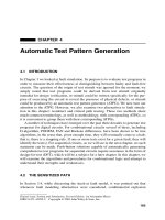
illustrated by means of the circuit in Figure 4.3. Consider the output of NOR gate B
SA0. Inputs I
2
and I
3
must be 0 in order to get a 1 on the output of B in the fault-free
circuit. In order for the fault to propagate through gate E, input I

1
must be 0. Hence
the output of E is 0 for the fault-free circuit, and it is 1 for the faulty circuit. In order
for E to be the controlling input to gate H, the other three inputs to H must be set to 0.
To get a 0 at the output of F, one of its inputs must be set to 1. Since the output of B
is SA0, input I
4
must be set to 1. The output of gate C then assumes the value 0 which,
together with the 0 on I
3
, causes the output of gate G to become 1. The sensitized path
is now inhibited, so there does not appear to be a test for the fault. But a test does exist.
The input assignment (0,0,0,0) will detect a SA0 fault at the output of gate B.
4.3 THE D-ALGORITHM
The inability to generate a test for the fault at the output of gate B in Figure 4.3
occurred because the sensitized path procedure always attempts to propagate fault
Figure 4.3 Effect of reconvergent fanout.
M
N
Q
P
I
1
I
2
I
3
I
4
A

B
C
D
E
F
G
H
THE D-ALGORITHM
171
symptoms through a single path. In the example it was necessary to make a choice
because of the presence of fanout. In fact, that was the problem with the first exam-
ple, that used Figure 4.1. It was not necessary to perform that last operation in which
I
5
was changed from 1 to 0. Even though the D and D canceled each other out at gate
N, the D at the output of gate M would have propagated through gate O and made it
to the output as a D. Rather than make a choice, the D-algorithm is capable of prop-
agating a sensitized signal through all paths when it encounters a net with fanout.
We start by formally defining the D-notation of Roth by means of the following
table.
3
The D simultaneously represents the signal value on the good circuit (GC)
and the faulted circuit (FC) according to the following table:
Conceptually, the D represents logic values on two superimposed circuits. When the
good circuit and the faulted circuit have the same value, the composite circuit value
will be 0 or 1. When they have different values, the composite circuit value will be
D, indicating a 1 on the good circuit and 0 on the faulted circuit, or D
, indicating a 0
on the good circuit and 1 on the faulted circuit.
At the output of gate B in Figure 4.3, where a SA0 fault was assigned, the fault-free

circuit must have logic value 1; therefore a D is assigned to that net. The goal is to
propagate this D to a primary output. Since the output of B drives two NOR gates, the
D is assigned to an input of gate E and to an input of gate F. Suppose we require that the
other input to both of these NOR gates be the nonblocking value; that is, we assign
I
1
= I
4
= 0. What value appears at the outputs of E and F? The inputs are 0 and D on
both NOR gates, and the D represents 1 on the good circuit and 0 on the faulted circuit.
So NOR gate inputs 0 and 1 are ORed together and inverted to give a 0 on the output of
the fault-free circuit, and NOR gate inputs 0 and 0 are ORed and inverted to give a 1 on
the output of the faulty circuit. Hence, the outputs of gates E and F are both D.
Two sensitized paths, both of which have the value D, are now converging on H.
If NOR gates D and G both have output 0, then the inputs to H are (0,0,0,0) for the
good circuit and (0,1,1,0) for the faulted circuit. Since H is a NOR gate, its output is
1 for the good circuit and 0 for the faulted circuit; that is, its output is a D. However,
we are not yet done. We need to obtain 0 from gates D and G. Since all of the inputs
are assigned, all we can do is inspect the circuit and hope that the input assignments
satisfy the requirement D = G = 0. Luckily, that turns out to be the case.
4.3.1 The D-Algorithm: An Analysis
A small example was analyzed rather quickly, and it was possible to deduce with lit-
tle difficulty what needed to be done at each step. A more rigorous framework will
FC
GC
01
00D
1D1
172
AUTOMATIC TEST PATTERN GENERATION

now be provided. We begin with a brief description of the cube theory that Roth
used to describe the D-algorithm.
A singular cube of a function is defined as an assignment
where the x
i
are inputs, the y
j
are outputs, and e
i
∈{0, 1, X}. A singular cube in
which all input coordinates are 0 or 1 is called a vertex. A vertex can be obtained
from a singular cube by converting all Xs on input coordinates to 0s and 1s.
A singular cube a contains the singular cube b if b can be obtained from a by
changing some of the Xs in a to 1s and 0s. Alternatively, a contains b if it contains
all of the vertices of b. The intersection of two singular cubes is the smallest singular
cube containing all of their common vertices. It is obtained through use of the inter-
section operator that operates on corresponding coordinates of two singular cubes
according to the following table:
The dash (—) denotes a conflict. If one singular cube has a 0 in a given position and
the other has a 1, then they are in conflict; the intersection does not exist. Two singu-
lar cubes are consistent if a conflict at their output intersections implies a conflict on
their input intersections. In terms of digital logic, this simply says that a stimulus
applied to a combinational logic circuit cannot produce both a 1 and a 0 on an out-
put. The term singular is used to denote the fact that there is a one-to-one mapping
between input and output parts of the cube. We will henceforth drop the term singu-
lar; it will be understood that we are talking about singular cubes. Furthermore, to
simplify notation, we will restrict our attention in what follows to single output
cubes, the definitions being easily generalized to the multiple output case.
A cover C is a set of pairwise consistent, nondegenerate cubes, all referring to the
same input and output variables. Given a function F, a cover of F is a cover C such

that each vertex v ∈ F is contained in some c ∈ C. A prime cube of a cover is one
that is not contained in any other c ∈ C. If the output part of a cube has the value 0,
the cube will be called a 0-point; if it has value 1, it will be called a 1-point; and if it
has value X (don’t care), it will be called an X-point. An extremal is a prime cube
that covers a 0-point or 1-point that no other prime cube covers.
Example The function can be represented by the cube of
Figure 4.4. The set of vertices for this cube is as follows:
I 01X
00— 0
1 — 11
X01X
x
1
… x
n
y
1
… y
m
,,,,,()e
1
e
2
… e
mn+
,, ,()=
Fa
0
a
1

a
0
a
2
+=
THE D-ALGORITHM
173

The following is a covering for the function which consists of prime cubes (asterisks
denote extremals):
The set of cubes for which the output is a 1 is denoted p
1
. Likewise, p
0
denotes the
set of cubes whose output is 0. The reader should verify that each vertex of F is
contained in at least one extremal. Two intersections follow:
In the first intersection the cube (0, 1, 1, 1) is the smallest cube that contains all
points common to the two vectors intersected. The second intersection is null. From
Figure 4.4 it can be seen that the two cubes have no points in common. The set of
extremals contains all of the vertices; hence it completely specifies the function for
all defined outputs.
The reader familiar with the terms “implicant” and “prime implicant” may note a
similarity between them and the cubes and extremals of cube theory. An implicant is
a product term that covers at least one 1-point of a function F and does not cover any
0-points. An implicant is prime if
1. For any other implicant there exists a 1-point covered by the first implicant
that is not covered by the second implicant, and
2. When any literal is deleted, the resulting product term is no longer an
implicant of the function.

a
0
a
1
a
2
F
0000
0011
0100
0111
1000
1010
1101
1111
*11X1



p
1
X111
*0 X 1 1
*10X0



p
0
X000

*0 X 0 0
X111 10X1
0X11 0X00
0111 —

174
AUTOMATIC TEST PATTERN GENERATION
Figure 4.4 Cube representation of a function.
Implicants and prime implicants deal with product terms that cover 1-points,
whereas cubes deal with both 1-points and 0-points. The cover corresponds to the
set of implicants for both the function F and its complement F
. The collection of
extremals corresponds to the set of prime implicants for both the function F and its
complement F
.
4.3.2 The Primitive D-Cubes of Failure
A primitive is an element that cannot be further subdivided; processing power is
built into the D-algorithm. Up to this point the basic switching gates have been
regarded as primitives. As we shall see, the D-algorithm can accommodate primi-
tives that are composites of several basic switching gates. A fault model for the
D-algorithm is called a primitive D-cube of failure (PDCF). The two-input AND
gate will be used to describe the procedure for generating a PDCF. We start with a
cover for the AND gate, in which the input vertices are numbered 1 and 2, and the
output vertex is number 3.
If input 1 is SA1, then the output is completely dependent on input 2. The cover then
becomes
123
000




p
0
010
100
111}p
1
123
000



f
0
100
011



f
1
111
(0,0,0) (0,0,1)
(1,0,1)
(1,1,1)(1,1,0)
(0,1,0)
(1,0,0)
(0,1,1)
(0,X,1)
a

0
a
2
a
1
(1,1,X)
(X,1,1)
THE D-ALGORITHM
175
(When referring to the faulted circuit, the set of 0-points is denoted as f
0
while the set
of 1-points is as f
1
.) We now have two distinct circuits. The first one produces an out-
put of 1 only when both inputs are at 1. The second circuit produces an output of 1
whenever the second input is a 1, regardless of the value applied to the first input. A
cursory examination of the two sets of vertices reveals an input combination, (0,1),
that causes a 0 output from the fault-free circuit and a 1 from the faulted circuit. The
vector (0,1) is clearly, then, a test for the presence of the SA1 fault on input 1.
Are there any other tests for input 1 SA1? The answer can be determined by per-
forming a point-by-point comparison of vertices from the two sets of vertices. In this
case, there is only one test for input 1 SA1. This test is the PDCF for the SA1 fault
on input 1 of the AND primitive. The comparison of vertices from the two sets can
be performed using the intersection table of the previous section. When we get to the
output, we do not flag it as a conflict; rather, we assign a D
, where D and D have the
meanings described previously.
If the two-input AND gate is faulted with its output SA1, the cover for this
faulted two-input AND gate becomes

There are three tests for the output SA1, and any of these tests can be chosen for the
fault. However, from the first two entries it is observed that the second input can be
either a 0 or a 1 (i.e., its value does not matter), suggesting the test (0, X). Likewise,
from the first and third entries it can be concluded that (X, 0) is a test for the fault.
The value of this observation lies in the fact that only one input needs to be assigned.
Can this be computed algorithmically?
Consider again the input SA1 fault for the two-input AND gate. The cover for the
good circuit can be described in terms of extremals. For the good circuit the cover is
For the faulted gate the cover is
123
001



f
1
011
101
111
123
0X0



p
0
X0 0
111}p
1
123

X0 0}f
0
X1 1}f
1
176
AUTOMATIC TEST PATTERN GENERATION
The vertex (0,1) is contained in the input parts of the cubes (0, X, 0) ∈ p
0
and (X, 1,1)
∈ f
1
. The input parts of these two cubes can be intersected to yield the original vertex
(0,1). The intersection of an element from p
0
with an element from f
1
has produced a
test for input 1 of the AND gate SA1. This, then, suggests the following general
method for finding test(s) for a particular fault:
1. Create a cover consisting of extremals for both the fault-free and faulted
circuits.
2. Intersect members of f
0
with members of p
1
.
3. Intersect members of f
1
with members of p
0

.
Since there must be at least one vertex that produces different outputs for the good
circuit and faulted circuit (why?), either step 2 or step 3 (or both) must result in a non-
empty intersection. Note that the intersections need not necessarily result in a vertex.
Example Consider the output of the two-input AND gate SA1. The cover f
1
con-
sists of the single cube (X, X, 1). Intersecting it with the extremals in p
0
results in the
two tests (0, X, D) and (X, 0, D). (When performing steps 2 and 3 above, only the
input parts are intersected.) 
PDCFs were developed for a rather elementary circuit, namely an AND gate. We
leave it as an exercise for the reader to develop PDCFs for other elementary gates
such as OR, NAND, NOR, and Invert. We point out that the technique for creating
PDCFs is quite general. Given a cover for a circuit G and its faulted counterpart, the
method just described can create a test for the circuit. As an example, consider the
AND-OR-Invert (AOI) of Figure 4.5. The circuit with input 1 SA1 is denoted G*.
The Karnaugh maps for G and G* are

Figure 4.5 AND-OR-Invert (AOI) circuit.
10 1
1
00 0
0
10 1
1
10 1
1
X

1
X
3
X
4
X
2
10 0
1
00 0
0
10 0
1
10 0
1
X
1
X
3
X
4
X
2
G
G*
G
X
1
X
2

Y
1
Y
2
THE D-ALGORITHM
177
The extremals for G and G* are
The complete set of intersections p
0
∩ f
1
and p
1
∩ f
0
yields
Either of these two vectors will distinguish between the fault-free circuit and the
circuit with input 1 SA1.
4.3.3 Propagation D-Cubes
The D-algorithm provides methods for processing circuits composed of a network
of primitives. Associated with each primitive is a set of rules for propagating tests
through it and for justifying test assignments from its outputs back to its inputs. Dur-
ing propagation a sensitized signal, D or D
, appears at one or more inputs to a prim-
itive, and the remaining inputs must be assigned logic values that cause the output to
be totally dependent on the sensitized signal. It is also assumed, in keeping with the
single-fault assumption, that the primitive through which the fault is propagating is
fault-free; that is, the fault of interest occurred elsewhere and the task is to drive it to
an observable output.
Since the goal is to drive a test through the primitive, a situation must be created

in which the response at the output of the primitive in the fault-free circuit is 1 and
the response at the output of the primitive in the faulted circuit is 0, or conversely.
This tells us that if the input part of the cube for the primitive in the fault-free circuit
is in p
0
, then the input part of the cube for the primitive in the faulted circuit must be
in p
1
, and vice versa. This suggests that we again want to perform intersections. We
will perform intersections, but the previous intersection table cannot be used
X
1
X
2
X
3
X
4
GX
1
X
2
X
3
X
4
G*
11XX0




p
0
X1 XX0



f
0
XX110 XX110
0X0X1



p
1
X0 0 X1



f
1
0XX01 X0X01
X00X1
X0X01
01 0 XD
01 X0 D
178
AUTOMATIC TEST PATTERN GENERATION
because it prohibited conflicts. We are now actually looking for conflicts so we use

the following table:
The row and column labels represent the values on input i of the first and second
cubes, respectively. Since elements from p
0
are intersected with elements from p
1
, a
conflict will always appear on the output. A conflict will also appear on at least one
input coordinate position. If all possible intersections are performed, a table of
entries called propagation D-cubes is created. Then, when a signal must propagate
through a primitive, a search is made through the table for an entry with D and D
values that match the signals on the input position(s) of the primitive through which
a signal is being propagated. That entry identifies the values that must occur on other
inputs to the circuit.
Example Using the cover for the AND-OR-Invert of Figure 4.5, and intersecting p
0
with p
1
, the following propagation D-cubes are obtained for the AND-OR-Invert:

There are actually 16 propagation D-cubes. The other eight are obtained by
intersecting p
1
with p
0
. They can also be obtained by exchanging D and D signals
on both the inputs and outputs. In actual practice it is often necessary to restrict the
propagation D-cube tables to contain only those propagation D-cubes having a
single D or D
among the inputs. That is because it is possible to have as many as

2
2n–1
propagation D-cubes for a function with n inputs. For a function with 6 inputs,
this could result in a table of 2048 entries if all single and multiple D and D signals
were maintained on the inputs. Multiple D and D values on the inputs are needed
much less frequently than single D or D
signals and can be created from the cover
when needed.
01X
00 D
0
1D1 1
X0 1 X
12 3 4 G
D1 0 X D
1D0 XD
D1 X 0 D
1DX0 D
0XD1 D
0X1 DD
X0 D 1 D
X0 1 D D

THE D-ALGORITHM
179
Figure 4.6 AOI with AND gate input.
4.3.4 Justification and Implication
We created a set of inputs for a primitive circuit and saw how to propagate the resulting
test through other logic in order to make the test visible at an output. Signal assignments
made to the outputs of primitives during the propagation phase must also be justi-

fied. Consider the circuit of Figure 4.6. It is the AND-OR-Invert with input 1 now
driven by an AND gate. We want to again test input X
1
for the SA1 fault. Therefore
input X
1
of the AOI must be 0. Because we are familiar with the behavior of the
AND gate, we can easily deduce that either input X
5
or X
6
must be 0 to get the
required 0 at X
1
. Alternatively, we can go to the cover for the AND gate and select an
entry from p
0
. The selected entry will tell us what values must be applied to the
inputs in order to get the required 0 on the output.
The selected entry may not always be acceptable. In Figure 4.7 we again consider
the AOI as a primitive. It is configured as a 2-to-1 multiplexer by virtue of the
inverter. If the goal is to create a test for a SA1 on the net labeled X
2
, then the first
step is to apply (1, 0, 0, X) to nets X
1
, X
2
, X
3

, and X
4
. These assignments must be
justified. Assuming the 1 on net X
1
can be justified, then the 0 assigned to net X
2
must be justified. When we examine the cover for the inverter, we find that we need
a 1 on the input. This requires a 1 on the output of the AND gate. We then seek to
justify the 0 on net X
3
, but it requires a 0 from the AND gate. A conflict exists. It is
obviously not possible to get a 0 and 1 simultaneously from the AND gate.
To resolve this conflict, an alternate decision must be made. Fortunately another
PDCF, (1, 0, X, 0), exists for the fault. With this alternate PDCF net, X
3
no longer
requires an assignment. The original PDCF (1, 0, 0, X) implied a 0 at the output of the
AND gate and hence to the input of the inverter. That in turn implied a 1 on the output
of the inverter and produced a conflict. Had the implications of the test (1, 0, 0, X)
been extended, the computations required to justify the assignment on net 1 could
have been avoided.

Figure 4.7 AOI as a multiplexer.
G
X
1
X
2
X

3
X
4
X
5
X
6
X
5
X
1
X
2
X
3
X
4
X
6
Comb.
logic
G
180
AUTOMATIC TEST PATTERN GENERATION
4.3.5 The D-Intersection
Covers, PDCFs, and propagation D-cubes have now been developed. These must be
used to create tests for circuits composed of numerous interconnected primitives.
This will be accomplished by means of the D-intersection that we define with the
help of another of our ubiquitous intersection tables.
The D-intersection table defines the results of a pairwise intersection of corre-

sponding elements of two vectors whose elements are members of the set {0, 1, D,
D
, X}. The elements represent the values on the inputs of a circuit as well as the
values on the outputs of individual primitives in the circuit.The dash (—) indicates a
conflict, in which case the intersection does not exist. We postpone discussion of
λ
and
µ
until later.
The D-intersections will be used to extend a sensitized path from the point of a
fault to the inputs and outputs of the circuit. The first step is to select a fault and
assign a PDCF. The propagation D-cubes and the cover are then used in conjunction
with the D-intersection table to form subsets of connected nets where we say that
two nets are connected if the values assigned to them are the direct result of (a) the
assignment of a PDCF or (b) a succession of one or more nontrivial D-intersections.
A nontrivial intersection requires that the vectors being intersected have at least
one common coordinate position in which neither of them has an X value.
The set of all connected nets forms a subcircuit called the test cube, also some-
times called a D-chain. Associated with a test cube are an activity vector and a
D-frontier. The activity vector consists of those nets of the test cube that (a) are out-
puts of the test cube and (b) have a value D or D
assigned.
The D-frontier is the set of gates with outputs not yet assigned that have one or
more input nets contained in the activity vector. The objective is to start with the
PDCF and form an expanding test cube via D-intersections between an existing test
cube and the propagation D-cubes and members of the primitive covers until the test
cube reaches the circuit inputs and outputs.
Example The D-algorithm will be used to create a test for the circuit in Figure 4.3.
Operations will be listed in tabular form, numbers will be assigned to relevant steps,
and we will refer to the step numbers as we explain the operations. The calculations

are shown in Figure 4.8.
D-
INTERSECTION
T
ABLE
01XDD
00— 0 ——
1 — 11——
X0 1 XDD
D —— D
µλ
D —— D
λµ
THE D-ALGORITHM
181
Figure 4.8 D-chain for Schneider’s counterexample.
In the first step a PDCF was assigned for a SA0 on the output of gate 6. It was then
propagated through gate 9. The intersection produced the result
µ
on the output of
gate 6. We now give the rules for processing the
µ
and
λ
symbols:
1. If one or more
µ
s occur, convert them to the corresponding D or D signals that
appear in the test cube and propagation D-cube.
2. If one or more

λ
s occur, complement all D and D signals in the propagation
D-cube, perform the intersection again, and convert the resulting
µ
s according
to rule 1.
3. if
µ
s and
λ
s both occur, the intersection is null.
In accordance with rule 1, the
µ
on the output of gate 6 is converted to a D.
Because gate 6 fans out to two gates, the activity vector consists of gates 6 and 9 and
the D-frontier consists of gates 10 and 12. We refrain from implying signals in this
example, choosing instead to propagate through gate 10 in step 4. We again produce
a
µ
which is converted to a D.
In step 6, propagation occurs through gate 12, producing a
λ
on gates 9 and 10. The
D and D signals in the propagation D-cube are complemented, and for convenience
the step is relabeled as step 6′. This results in
µ
appearing on gates 9 and 10. These are
then both converted to D in step 7. In this step a multiple path was propagated through
123456789
X

X0 0 XDXXX
0
D
10 11 12
1.
2.
X
XX
000XXXXm
m
mm
X
XX
0
00
XXDXX
XX
X
3.
D
D
D
D
D
D
D
D
D
DD
D

D D
D
D
DD
DD04.
0000X XX XX
000 0XDXX XX
0
DD
0
000 0XDX 0 ll0
0000XDX0 D0
X10
0000XD1 D00
X10
00001D10 D0
5.
6.
7.
8.
9.
10.
000 0 XDXX X
X
0
DD
0
0000XD DX0 0
5.
6.

182
AUTOMATIC TEST PATTERN GENERATION
gate 12. The values at the inputs to gate 12 are (0, 0, 0, 0) for the fault-free circuit and
(0, 1, 1, 0) for the faulted circuit. If propagation D-cubes with multiple D and D sig-
nals are not stored in the propagation D-cube table, it would be necessary to create the
required propagation D-cube, using the cover consisting of vertices.
Finally, having propagated a signal to the output, assignments to internal gates
must now be justified. In step 8 the assignment of a 0 to gate 11 is justified by assign-
ing a 1 to gate 7 and an X to input 3. In step 9 the same is done for gate 8. It is also
necessary to justify the values assigned to gates 7 and 5, but at this stage it merely
requires confirming that the values on their inputs satisfy the requirements on the out-
puts, since there are no more assignments that can be made. The final test cube is
shown in line number 10. 
Fortunately, it was not necessary to invoke rule 3,
µ
and
λ
did not occur simulta-
neously. If they had, then it indicates that the test cube and the propagation D-cube
have D and D signals in more than one common position. Furthermore, some of the
signals were in agreement and some were in conflict. Therefore, complementing all
D and D signals in the propagation D-cube will not resolve the conflict.
The D-algorithm is sometimes referred to as a two-dimensional algorithm, in
contrast to path sensitization, which has been characterized as one-dimensional.
Strictly speaking, the path sensitization method is not even an algorithm, but, rather,
a procedure. The distinction lies in the fact that an algorithm can always find a solu-
tion if a solution exists. In other respects they are similar, since both an algorithm
and a procedure can be programmed, such that a next step or a criterion for termina-
tion always exists. The reader is cautioned to note that authors are not consistent on
the usage of these terms, some calling an algorithm that which is more accurately

called a procedure. While we may not always strictly adhere to this distinction, the
reader should be aware that when an author sets out to demonstrate that his method
is an algorithm, he must show that it will find a solution whenever a solution exists.
The proof that the D-algorithm is an algorithm consists of showing that if a test
cube c(T,F) exists for failure F, the test cube c(T,F) must be contained in a PDCF.
Also, a test cube must contain a connected chain of coordinates having values D or
D linking the output of the faulted gate to a primary output. Given a particular gate
through which the test passes on its way to an output, the test cube c(T,F) must be
contained in some propagation cube of the gate in question since the propagation
D-cubes are constructed so as to define all possible combinations by which a test can
be propagated through the gate. Finally, the fact that all propagation D-cubes are
candidates for intersection, including those with multiple propagation paths, assures
that all possible chains can be constructed, implying that, given a particular test, the
D-algorithm will find that test (if it does not find some other test first).
4.4 TESTDETECT
The D-algorithm is used to construct sensitized paths extending from fault origins to
primary outputs. The D-notation keeps track of values along the way, and the tables
TESTDETECT
183
that define operations on pairs of logic signals and/or D-symbols make it possible to
evaluate progress, as well as to identify nodes where signals occur that block or
impede the progress of the D-signals. Using this same D-notation, Paul Roth devel-
oped a procedure, called Testdetect, that relies on D-signals to determine which
faults are detected by a given input vector.
4
To understand the operation of Testdetect, consider the circuit in Figure 4.1. The
input pattern I
1
, I
2

, I
3
, I
4
, I
5
= (0, 0, 1, 0, 0) is applied to the circuit. This input pattern
results in a 0 at the output Z. Obviously, if the output is SA1, the fault will be detected.
The outputs of gates K, L, N, and O are all 1s for the fault-free circuit. If the output of
any of these gates is SA0, that fault will cause the output to assume the value 1; hence
those SA0 faults will also be detected. It is possible to continue tracing back toward
the inputs, from any fault that is detected, to identify other faults that will be detected.
For example, if an SA0 on the output of gate L is detectable, then any fault on the input
of L that causes its output to assume the value 0 is also detectable.
Testdetect formalizes this approach. It selects a fault and determines whether a
D-chain can be extended from this fault to an observable output. However, in this
inverse D-algorithm, all signal values are fixed. The objective is not to create a test
but rather, having created a test, to determine what other faults are detected by the
input vector. Therefore, the object is to determine, for a given fault, if its effects
propagate through a series of gates, eventually reaching an output.
A D-list keeps track of gates in the D-frontier while progressing toward primary
outputs. A gate is selected from the D-list, and it is determined whether the fault will
propagate through the gate. If not, then the D-chain has died on that path; and if the
D-list is empty, the fault will not be detected by that test vector. If the fault does
propagate through the gate, then the gate or gates in the fanout from that gate are
placed in the D-list. This continues until either
1. A primary output is encountered, or
2. The D-list becomes empty.
A third criteria for stopping exists:
Lemma 4.1 If at any stage in the computation for failure F, the D-frontier reduces

to a single net L and there is no reconvergent fanout beyond the D-frontier, then F is
testable iff if L is testable.
5
Rules for determining whether or not a fault propagates through an element are the
same as those used in the D-algorithm. For an AND gate with a D or D on an input (or
inputs), if the other inputs are all 1s, then the D or D
will propagate to the output of
the gate. In general, if the good circuit signal causes a 1 (0) on the output of the gate
and the fault causes a 0 (1), then the fault signal propagates to the output of the gate.
Example For the circuit of Figure 4.1, with the inputs I
1
,I
2
,I
3
,I
4
,I
5
= (0,0,1,0,0), the
output of gate L has a 1. An SA0 on the output of L produces a D, which shows up at
the output of the circuit as a D
. Hence the SA0 is detected. If the upper input to gate
L is SA0, then (D
,0) produces a D on the output of L. By the lemma, the fault is
detected. However, an SA0 on the output of gate D must be analyzed all the way to
the output because there are two gates, J and L, in its D-list.
184
AUTOMATIC TEST PATTERN GENERATION
A D is assigned to the output of gate D, indicating a SA0 on its output, and J and

L are placed in the D-list. We assume that the circuit has been rank-ordered, and we
require that when there are two or more entries in the D-list, the lower numbered gate
to be selected first. (Why?) Therefore, gate J is selected for processing. The inputs to
gate J are (0,0,1,D). Since the 1 on the third input is inverted at the input, the output
of J is a D. This causes K to be placed in the D-list. Since it precedes L (alphabeti-
cally), it is processed next. The D from gate J, together with the 0s on its other inputs,
causes a D to appear on its output. Gate L is processed next, and a D appears on its
output. The subcircuit consisting of M, N, O, and P represents an exclusive-OR, so
the D signals appearing at the inputs to this subcircuit cancel at the output. Hence the
fault on the output of gate 9 is not detected by this test pattern. 
The failure to detect a fault on the output of gate D, despite the fact that it drives
a gate on which faults are detected, is caused by reconvergence of two sensitized
paths that cancel each other out. If there were no problems with reconverging logic,
Testdetect could run quite rapidly and work straight from the outputs back to the
inputs. However, reconvergent fanout necessitates that all fanout branches be exam-
ined. In the example, we looked at a situation where a pair of D-chains diverged at
the D-frontier. It is possible to have a D-frontier with a single element that is detect-
able and still not have a detectable fault. Such a condition is illustrated in Figure 4.9.
With the input combination 1, 2, 3 = (1, 0, 0), a fault on the output of gate 5 is detect-
able. But, consider what happens if the input combination 1, 2, 3 = (1, D
, 0) is applied
to test for an SA1 at input 2. This causes a D to appear at the output of gate 5 and causes
a D to appear at the output of gate 4. With D and D on its inputs, the output of gate 6 is
a 0. We are left with only gate 5 in the D-list, and that was previously determined to be
detectable by the applied pattern, yet the SA1 at primary input 2 is not detectable
because the 0 on the output of gate 6 prevents the D at gate 5 from reaching the output.
4.5 THE SUBSCRIPTED D-ALGORITHM
Given an AND gate or an OR gate, for each input fault to be tested the D-algorithm
must recompute a propagation path from that gate to a primary output. This effort
becomes increasingly redundant for circuits in which many gates have a large num-

ber of inputs. Elimination of these redundant computations is one of the objectives
of the subscripted D-algorithm, or A-algorithm (AALG).
6
Figure 4.9 Recombining sensitized paths.
6
1
2
3
7
1
0
0
0
D
D
D
D
4
5
8
THE SUBSCRIPTED D-ALGORITHM
185
The AALG goes farther, however. Whereas the D-algorithm selects a single fault
and justifies fixed binary values on the inputs of the corresponding gate, AALG
simultaneously justifies symbolic assignments on all inputs in a process called back-
propagation. The first step in this process is to select a gate and assign the symbol
D
0
to its output. This symbol is propagated to a primary output using the same
forward-propagation techniques employed in the D-algorithm. If the gate has m

inputs, then a symbol D
i
, 1 ≤ i ≤ m, is assigned to each of its inputs.The D
i
are called
flexible signals; they may represent 0 or 1, depending on what values are required
for a particular test.
After the D
0
signal has been successfully propagated to an output, all of the D
i
are back-propagated to primary inputs. If the back-propagation is completely suc-
cessful, then tests for the output fault and all of the gate input faults can be computed
simply by inspecting values at the primary inputs. This is illustrated in the circuit of
Figure 4.10, where the input vector I has value I = (X, 0, D
1
, D
2
, 0, 0).
This vector is interpreted by referring back to the gate where the D
i
originated. A
test for the output of gate 16 SA0 requires both of its inputs to be 1, that is, D
1
,
D
2
= (1, 1), which requires inputs 3, 4 = (1, 0). Tests for SA1 on inputs 1 and 2 of
gate 16 require D
1

, D
2
= (0, 1) and (1, 0), respectively. Therefore, the tests for these
three faults are
(X, 0, 1, 0, 0, 0)
(X, 0, 0, 0, 0, 0)
(X, 0, 1, 1, 0, 0)
The input assignments are not unique. For example, the input vector I could have
been assigned the values (D
1
, 1, X, D
2
, 1, 1). Several other possibilities exist,
depending on choices made at gates where decisions were required during
back-propagation.
Figure 4.10 Illustrating the subscripted D-algorithm.
D
0
D
1
D
2
D
2
D
1
D
1
1
2

3
5
6
X
0
0
15
7
4
0
0
0
9
10
11
12
13
14
16
17
18
8
186
AUTOMATIC TEST PATTERN GENERATION
We now discuss the rules for back-propagation. Basically, each D
i
is back-
propagated toward the inputs along as many paths as possible. This is done through
replication. When symbolically propagating back through an element, the symbol D
i

at the output is replicated at the inputs, according to the following rules:
1. If a gate inverts a signal, then the inputs are assigned D
i
.
2. D
i
(or D
i
) is replicated at all inputs if no input has been previously assigned.
3. D
i
can be replicated at some inputs if all others are assigned noncontrolling
values.
Example Given a three-input NAND gate, with one of its inputs assigned a logic 1,
and D
j
assigned to its output during back-propagation, the remaining two inputs are
assigned D
j
. 
This proliferation of D
i
signals enhances the likelihood of establishing a sensitized
path from one or more primary inputs to input i of the gate presently being tested, in
contrast to propagation of a single replica, which may require considerable back-
tracking* in response to conflicts. However, it is still possible to encounter conflicts.
In fact, with flexible signals increasing exponentially in number as progress continues
toward the inputs, conflicts are virtually inevitable in any realistic circuit. Efficient
handling of conflicts is imperative if performance is to be realized.
A conflict can occur during back-propagation as a result of a signal D

i
and a con-
flicting value of that same signal attempting to control a gate, or as a result of two
different signals D
i
and D
j
attempting to control a gate, or a conflict may occur at a
gate with fanout if two or more signal paths reconverge at the gate and one of the
paths has a flexible signal while another has a fixed binary value.
The situation in which conflicting values of the same flexible signal try to control
a gate is illustrated in the upper path of Figure 4.10. The assignment of D
1
on the
output of gate 13 during back-propagation initially results in the replication of D
1
on
each of its inputs, hence on the outputs of gates 9 and 10. Back-propagation then
produces replicas of D
1
on both inputs of gates 9 and 10. However, we are now faced
with the prospect of flexible signal D
1
on both the input and output of inverter I
7
.
This conflict can be resolved by assigning a 0 or 1 to the output of gate 7. Choosing
a 1 forces 0s on the input of gate 7 and the lower input of gate 9, which forces a 0 on
the output of gate 9 and also causes the upper input to gate 9 to be reassigned to X.
The conflict between flexible signals D

j
and D
k
can be illustrated by assigning D
0
to gate 14. Forward propagation and justification along the upper path are the same
as in the D-algorithm. We therefore restrict our attention to the consequences of a D
0
on gate 14. This requires D
1
and D
2
on the inputs to gate 14. Back-propagation then
attempts to assign both D
1
and D
2
to the output of gate 8. Again, the conflict is
*In the discussion that follows, the terms backtracing and backtracking will be used. It is easy to confuse
them. Backtracing is the process of working backward in the circuit model, while backtracking is the pro-
cess of correcting for a conflict between node values.
7
THE SUBSCRIPTED D-ALGORITHM
187
resolved by assigning a fixed binary value to the output of gate 8. If a 1 is assigned,
then one of the inputs must be set to 0. However, the other flexible signal can still be
instantiated.
Generally, when an input must be set to a controlling value—for example, a 0 on
an input to an AND or NAND gate—it is usually preferable to choose the input that
is easiest to control. However, in the present case an additional criterion may exist. If

a fault on one of the two inputs to gate 14 has already been detected, then the flexi-
ble signal D
1
or D
2
corresponding to the undetected input fault can be favored when
a choice must be made. When D
1
and D
2
converge at the output of gate 8, if it is
found that the upper input to gate 14 has already been tested, then D
1
can be purged
by assigning a 0 to the upper input of gate 8.
When a conflict occurs, its resolution usually requires that segments of D
i
chains
be deleted. AALG accomplishes this with functions called DROPIT and DRBACK.
8
DROPIT purges a chain segment when the end closest to the primary inputs is
known. It works forward toward the gate under test. It must examine fanouts as it
progresses, so if two converging paths both have flexible signals, then both chain
segments must be deleted. When a flexible signal is deleted, it may be replaced by a
fixed binary signal. This signal, when assigned to the input of a gate, may be a con-
trolling value for that gate and thus implies a logic value on the output. In that case,
the output must be further traced to the input of the gate(s) in its fanout to determine
whether this output value is a controlling value at the input of the gate in its fanout.
When D
0

was assigned to the output of gate 14, a conflict occurred at gate 8, so a 1
was assigned to its output, which required a 0 on one of its inputs. Primary input 6
was chosen. This required that the D
2
chain from P.I. 6 to the input of gate 14 be
purged. A 0 on P.I. 6 implies a 0 on the output of gate 12, so the flexible signal D
2
ini-
tially assigned at the output of gate 12 must be purged and the path traced another
level. At gate 14 the enabling signal 0 is assigned to the lower input and the flexible
signal D
1
is assigned to the upper input. Therefore DROPIT can stop at that point.
If D
j
controls the output and one or more D
i
control the inputs, it may be desir-
able to propagate D
j
toward the inputs and purge the D
i
signals. In that case the end
of the chain farthest from the PIs is known and DRBACK purges the chain. Working
back toward the PIs, it may have to purge a considerable number of flexible signals
since the signals were originally replicated when working toward the inputs.
The functions DROPIT and DRBACK are not always invoked independently of
one another. When DROPIT is purging flexible signals and replacing them with
fixed binary signals, it may be necessary to invoke DRBACK to purge other chain
segments. This is seen in the upper branch of the circuit in Figure 4.10. Primary

input 2 was assigned a 0 because of a conflict. Therefore DROPIT, working for-
ward from primary input 2, purges D
1
and replaces it with a 0. The 0 on the lower
input of gate 9 blocks the gate and therefore DRBACK must pick up the chain seg-
ment on the upper input and delete it back to input 1 and replace it with X. Then
DROPIT regains control and proceeds forward. The 0 on the input of gate 7
implies a 0 on the output and hence a 0 on the input to gate 13. Since a 0 on an OR
gate is not a controlling value, the forward purge can stop, leaving gate 13 with
(0, D
1
) on its inputs.
188
AUTOMATIC TEST PATTERN GENERATION
To help identify and purge unwanted chain segments, flexible signals are never
implied forward to primary outputs during back-propagation. As an example, in
Figure 4.10, when back-propagating from gate 9 toward primary inputs, any assign-
ment to primary input 2 will necessarily imply the inverse signal on the output of
gate 7. However, if the flexible signal is assigned, then at some later point DROPIT
may go unnecessarily along signal paths, deleting flexible signals and replacing
them with controlling logic values where it may be unnecessary.
In measurements of performance, it has been found that AALG creates an input
pattern with flexible signals in about the same time that the D-algorithm generates a
single pattern. Overall time comparison for typical circuits shows that it frequently
processes a circuit in about 30% of the time required by the D-algorithm. AALG is
especially efficient, for reasons explained earlier, when working on circuits that have
gates with large numbers of inputs, as is sometimes the case with programmable
logic arrays (PLAs). The efficiency of AALG can be enhanced by first selecting pri-
mary outputs and then selecting gates with large numbers of inputs. Gates for which
the output has not yet been tested are chosen next since they usually indicate regions

where fault processing has not yet occurred. Finally, scattered faults are processed.
On those faults AALG occasionally defaults to the conventional D-algorithm.
4.6 PODEM
The D-algorithm selects a fault from within a circuit and works outward from that
fault back to primary inputs and forward to primary outputs, propagating, justifying
and implicating logic assignments along the way. In circuits that rely heavily on
reconvergent fanout, such as parity checkers and error detection and correction
(EDAC) circuits, the D-algorithm may encounter a significant number of conflicting
assignments. When that happens it must find a node where an arbitrary choice was
made and choose an alternate assignment. This can be very CPU and/or memory
intensive, depending on how many conflicts occur and how they are handled.
PODEM (path-oriented decision making)
9
reduces the number of remade deci-
sions by selecting a fault and assigning logic values directly at the circuit inputs to
create a test. Much of its efficiency results from its ability to exploit the fact that sig-
nal polarity along sensitized paths is irrelevant. For example, when the D-algorithm
propagates a D or D through an XOR, it assigns a 1 or 0 to the other input, the
choice being arbitrary and often depending on how the software was coded. It may
then go to great lengths to justify that choice, despite the fact that either choice is
equally effective, and the chosen value may eventually produce a conflict, necessi-
tating a remade decision. PODEM, as we shall see, implicitly propagates through
the XOR, eliminating the need to make a choice at the other input, thus obviating the
need to make or alter a decision.
PODEM begins by initializing the circuit to Xs. A fault is chosen, and PODEM
backs up through the logic until it arrives at a primary input, where it assigns a
binary value, 0 or 1. Implications of this assignment are propagated forward. If
either of the following propositions is true, the assignment is rejected.
PODEM
189

1. The net for the selected stuck fault has the same logic value as the stuck fault.
2. There is no signal path from an internal net to a primary output such that the
internal net has value D or D
and all other nets on the signal path are at X.
Proposition 1 excludes input combinations that cause the fault-free circuit to assume
the same value as the stuck-at value at the site of the fault. Proposition 2 rejects
input combinations that block all possible paths from the fault to the outputs. If the
test is not complete and if there is no path to an output that is free to be assigned,
then there is no way to propagate a test to an output.
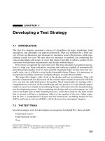
When PODEM makes assignments to primary inputs, it employs a branch-and-
bound method.
10
This process is represented by the tree illustrated in Figure 4.11.
An assignment is made to a primary input and is implied forward. If the assignment
does not violate proposition 1 or 2, it is retained and a branch is added to the tree. If
a violation occurs, the assignment is rejected and the node is flagged to indicate that
one value had been unsuccessfully tried. The tree is thus bounded. If the node had
been previously flagged, then it is completely rejected and it becomes necessary to
back up in the tree until an unflagged node is encountered, at which point the alter-
nate value is implied. The process continues until a successful test is created or the
process returns to the start node and both choices have been tried. If that occurs, it is
concluded that a test does not exist. The criterion for a successful test is the same as
that employed by the D-algorithm, namely, that a D or D
has propagated from the
point of a fault to a primary output.
If PODEM rejects the initial assignment to the ith input selected, and if there are n
primary inputs, then 2
n–i
combinations have been eliminated from further consider-
ation. If the initial assignment to the first primary input is rejected, then the number of

Figure 4.11 Branch-and-bound without backtrace.
PI
4
= 1
PI
3
= 0
PI
2
= 1
PI
1
= 1PI
1
= 0
PI
2
= 0
PI
5
= 0
PI
4
= 0
SUCCESS
All PIs initially
set to X
}{
START