Logic kỹ thuật số thử nghiệm và mô phỏng P5

233

Digital Logic Testing and Simulation

,

Second Edition

, by Alexander Miczo
ISBN 0-471-43995-9 Copyright © 2003 John Wiley & Sons, Inc.

CHAPTER 5

Sequential Logic Test

5.1 INTRODUCTION

The previous chapter examined methods for creating sensitized paths in combina-
tional logic extending from stuck-at faults on logic gates to observable outputs. We
now attempt to create tests for sequential circuits where the outputs are a function
not just of present inputs but of past inputs as well. The objective will be the same:
to create a sensitized path from the point where a fault occurs to an observable out-
put. However, there are new factors that must be taken into consideration. A sensi-
tized path must now be propagated not only through logic operators, but also
through an entirely new dimension—time. The time dimension may be discrete, as
in synchronous logic, or it may be continuous, as in asynchronous logic.
The time dimension was ignored when creating tests for faults in combinational
logic. It was implicitly assumed that the output response would stabilize before
being measured with test equipment, and it was generally assumed that each test pat-
tern was independent of its predecessors. As will be seen, the effects of time cannot
be ignored, because this added dimension greatly influences the results of test pat-

tern generation and can complicate, by orders of magnitude, the problem of creating
tests. Assumptions about circuit behavior must be carefully analyzed to determine
the circumstances under which they prevail.

5.2 TEST PROBLEMS CAUSED BY SEQUENTIAL LOGIC

Two factors complicate the task of creating tests for sequential logic: memory and
circuit delay. In sequential circuits the signals must not only be logically correct, but
must also occur in the correct time sequence relative to other signals. The test prob-
lem is further complicated by the fact that aberrant behavior can occur in sequential
circuits when individual discrete components are all fault-free and conform to their
manufacturer’s specifications. We first consider problems caused by the presence of
memory, and then we examine the effects of circuit delay on the test generation
problem.

234

SEQUENTIAL LOGIC TEST

5.2.1 The Effects of Memory

In the first chapter it was pointed out that, for combinational circuits, it was possible
(but not necessarily reasonable) to create a complete test for logic faults by applying
all possible binary combinations to the inputs of a circuit. That, as we shall see, is
not true for circuits with memory. They may not only require more than 2

n

tests, but
are also sensitive to the

order

in which stimuli are applied.

Test Vector Ordering

The effects of memory can be seen from analysis of the
cross-coupled NAND latch [cf. Figure 2.3(b)]. Four faults will be considered, these
being the input SA1 faults on each of the two NAND gates (numbering is from top
to bottom in the diagram). All four possible binary combinations are applied to the
inputs in ascending order—that is, in the sequence (Set
, Reset) = {(0,0), (0,1), (1,0),
(1,1)}. We get the following response for the fault-free circuit (FF) and the circuit
corresponding to each of the four input SA1 faults.
In this table, fault number 2 responds to the sequence of input vectors with an output
response that exactly matches the fault-free circuit response. Clearly, this sequence
of inputs will not distinguish between the fault-free circuit and a circuit with input 2
SA1.
The sequence is now applied in the exact opposite order. We get:

The Indeterminate Value

When the four input combinations are applied in
reverse order, question marks appear in some table positions. What is their signifi-
cance? To answer this question, we take note of a situation that did not exist when
dealing only with combinational logic; the cross-coupled NAND latch has

memory

.
By virtue of feedback present in the circuit, it is able to remember the value of a sig-
nal that was applied to the set input even after that signal is removed.
Input Output
Set
Reset FF1234
0 0 10111
0 1 10111
1 0 00001
1 1 00011
Input Output
Set
Reset FF1234
11??01?
1 0 0000?
0 1 10111
0 0 10111

TEST PROBLEMS CAUSED BY SEQUENTIAL LOGIC

235

Because of the feedback, neither the Set
nor the Reset line need be held low any
longer than necessary to effectively latch the circuit. However, when power is first
applied to the circuit, it is not known what value is contained in the latch. How can
circuit behavior be simulated when it is not known what value is contained in its
memory?
In real circuits, memory elements such as latches and flip-flops have indetermi-
nate values when power is first applied. The contents of these elements remain

indeterminate until the latch or flip-flop is either set or reset to a known value. In a
simulation model this condition is imitated by initializing circuit elements to the
indeterminate X state. Then, as seen in Chapter 2, some signal values can drive a
logic element to a known state despite the presence of indeterminate values on
other inputs. For example, the AND gate in Figure 2.1(c) responds with a 0 when
any single input receives a 0, regardless of what values are present on other
inputs. However, if a 1 is applied while all other inputs are at X, the output
remains at X.
Returning to the latch, the first sequence began by applying 0s to both inputs,
while the second sequence began by applying 1s to both inputs. In both cases the
internal nets were initially indeterminate. The 0s in the first sequence were able to
drive the latch to a known state, making it possible to immediately distinguish
between correct and incorrect response. When applying the patterns in reverse order,
it took longer to drive the latch into a state where good circuit response could be dis-
tinguished from faulty circuit response. As a result, only one of the four faults is
detected, namely, fault 1. Circuits with faults 2 and 3 agree with the good circuit
response in all instances where the good circuit has a known response. On the first
pattern the good circuit response is indeterminate and the circuit with fault 2
responds with a 0. The circuit with fault 3 responds with a 1. Since it is not known
what value to expect from the good circuit, there is no way to decide whether the
faulted circuits are responding correctly.
Faulted circuit 4 presents an additional complication. Its response is indetermi-
nate for both the first and second patterns. However, because the good circuit has a
known response to pattern 2, we do know what to look for in the good circuit,
namely, the value 0. Therefore, if a NAND latch is being tested with the second set
of stimuli, and it is faulted with input 4 SA1, it might come up initially with a 0 on
its output when power is applied to the circuit, in which case the fault is not
detected, or it could come up with a 1, in which case the fault will be detected.

Oscillations

Another complication resulting from the presence of memory is
oscillations. Suppose that we first apply the test vector (0,0) to the cross-coupled
NAND latch. Both NAND gates respond with a logic 1 on their outputs. We then
apply the combination (1,1) to the inputs. Now there are 1s on both inputs to each of
the two NAND gates—but not for long. The NAND gates transform these 1s into 0s
on the outputs. The 0s then show up on the NAND inputs and cause the NAND out-
puts to go to 1s. The cycle is repetitive; the latch is oscillating. We do not know what
value to expect on the NAND gate outputs; the latch may continue to oscillate until a
different stimulus is applied to the inputs or the oscillations may eventually subside.

236

SEQUENTIAL LOGIC TEST

If the oscillations do subside, there is no practical way to predict, from a logic
description of the circuit, the final state into which the latch settles. Therefore, the
NAND outputs are set to the indeterminate X.

Probable Detected Faults

When we analyzed the effectiveness of binary
sequences applied to the NAND latch in descending order, we could not claim with
certainty that stuck-at fault number 4 would be detected. Fortunately, that fault is
detected when the vectors are applied in ascending order. In other circuits the ambi-
guity remains. In Figure 2.4(b) the Data input is complemented and both true and
complement values are applied to the latch. Barring the presence of a fault, the latch
will not oscillate. However, when attempting to create a test for the circuit, we
encounter another problem. If the Enable
signal is SA1, the output of the inverter

driven by Enable
is permanently at 0 and the NAND gates driven by the inverter are
permanently in a 1 state; hence the faulted latch cannot be initialized to a known
state. Indeterminate states were set on the latch nodes prior to the start of test pattern
generation and the states remain indeterminate for the faulted circuit. If power is
applied to the fault-free and faulted latches, the circuits may just happen to come up
in the same state.
The problem just described is inherent in any finite-state machine (FSM). The
FSM is characterized by a set of states

Q

= {

q

1

,

q

2

, ...,

q

s

}, a set of input stimuli

I

= {

i

1

,

i

2

, ...,

i

n

}, another set

Y

= {

y

1

,

y

2

, ...,

y

m

} of output responses, and a pair of
mappings

M

:

Q



×



I

→

Q
Z

:

Q



×



I



→

Y

These mappings define the next state transition and the output behavior in response
to any particular input stimulus. These mappings assume knowledge of the current
state of the FSM at the time the stimulus is applied. When the initial stimulus is
applied, that state is unknown unless some independent means such as a reset exists

for driving the FSM into a known state.
In general, if there is no independent means for initializing an FSM, and if the
Clock or Enable input is faulty, then it is not possible to apply just a single stimu-
lus to the FSM and detect the presence of that fault. One approach used in industry
is to mark a fault as a

probable detect

if the fault-free circuit drives an output pin
to a known logic state and the fault causes that same pin to assume an unknown
state.
The industry is not in complete agreement concerning the classification of proba-
ble detected faults. While some test engineers maintain that such a fault is likely to
eventually become detected, others argue that it should remain classified as undetec-
ted, and still others prefer to view it as a probable detect. If the probable detected
fault is marked as detected, then there is a concern that an ATPG may be designed to
ignore the fault and not try to create a test for it in those situations where a test
exists.

TEST PROBLEMS CAUSED BY SEQUENTIAL LOGIC

237

Figure 5.1

Initialization problem.

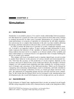
The Initialization Problem

Consider the circuit of Figure 5.1. During simula-

tion, circuit operation begins with the D flip-flop in an unknown state. In normal
operation, when the input combination

A

=

B

=

C

= 0 is applied and the flip-flop is
clocked, the

Q

output switches to 0. The flip-flop can then be clocked a second time
to obtain a test for the lower input of gate 3 SA1. If it is SA1, the expected value is

Q

= 1; and if it is fault-free, the expected value is

Q

= 0.
Unfortunately, the test has a serious flaw! If the lower input to gate 3 is SA1, the
output of the flip-flop at the end of the first clock period is indeterminate because the

value at the middle input to gate 3 is initially indeterminate. It is driven by the flip-
flop that has an indeterminate value. After a second clock pulse the value at

Q

will
remain at X; hence it may agree with the good circuit response despite the presence
of the fault. The fallacy lies in assuming correct circuit behavior when setting up the
flip-flop for the test. We depended upon correct behavior of the very net that we are
attempting to test when setting up a test to detect a fault on that net.
To correctly establish a test, it is necessary to assume an indeterminate value from
the flip-flop. Then, from the D-algorithm, we know that the flip-flop must be driven
into the 0 state, without depending on the input to gate 3 that is driven by the flip-
flop. The flip-flop value can then be used in conjunction with the inputs to test for
the SA1 on the lower input of gate 3. In this instance, we can set

A

=

C

= 0,

B

= 1.
Then a 1 can be clocked into the flip-flop from gate 2. This produces a 0 on the out-
put of the flip-flop which can then be used with the assignment

A

=

B

= 0 to clock a
0 into the flip-flop. Now, with

Q

= 0 and

A

=

B

=

C

= 0, another clock causes D
to
appear on the output of the flip-flop.
Notice that input

C

was used, but it was used to set up gate 2. If input

C

were
faulted in such a way as to affect both gates 2 and 3, then it could not have been used
to set up the test.

5.2.2 Timing Considerations

Until now we have assumed that erroneous behavior on circuit outputs was the result
of

logic

faults. Those faults generally result from actual physical defects such as
opens or shorts, or incorrect fabrication such as an incorrect connection or a wrong
Q
A
B
C
1
2
3
4
D
F
Clock
AF
0

C
0
Q
1
Q
10
SA1
B
0
1
0
1

238

SEQUENTIAL LOGIC TEST

component. Unfortunately, this assumption, while convenient, is an oversimplifica-
tion. An error may indeed be a result of one or more logic faults, but it may also be
the case that an error occurs and none of the above situations exists.
Defects exist that can prevent an element from behaving in accordance with its
specifications. Faults that affect the performance of a circuit are referred to as

para-
metric

faults, in contrast to the logic faults that have been considered up to this
point. Parametric faults can affect voltage and current levels, and they can affect
gain and switching speed of a circuit. Parametric faults in components can result
from improper fabrication or from degradation as a consequence of a normal aging

process. Environmental conditions such as temperature extremes, humidity, or
mechanical vibration can accelerate the degradation process.
Design oversights can produce symptoms similar to parametric faults. Design
problems include failure to take into account wire lengths, loading of devices, inad-
equate decoupling, and failure to consider worst-case conditions such as maximum
or minimum voltages or temperatures over which a device may be required to oper-
ate. It is possible that none of these factors may cause an error in a particular design
in a well-controlled environment, and yet any of these factors can destabilize a cir-
cuit that is operating under adverse conditions. Relative timing between signal paths
or the ability of the circuit to drive other circuits could be affected.
Intermittent errors are particularly insidious because of their rather elusive
nature, appearing only under particular combinations of circumstances. For exam-
ple, a logic board may be designed for nominal signal delay for each component as a
safety margin. Statistically, the delays should seldom accumulate so as to exceed a
critical threshold. However, as with any statistical expectation, there will occasion-
ally be a circuit that does exceed the maximum permissible value. Worse still, it may
work well at nominal voltages and /or temperatures and fail only when voltages and/
or temperatures stray from their nominal value. A new board substituted for the orig-
inal board may be closer to tolerance and work well under the degraded voltage and/
or temperature conditions. The original board may then, when checked at a depot or
a board tester under ideal operating conditions, test satisfactorily.
Consider the effects of timing variations on the delay flip-flop of Figure 2.7. Cor-
rect operation of the flip-flop requires that the designer observe minimal setup and
hold times. If propagation delay along a signal path to the Data input of the flip-flop
is greater than estimated by the designer, or if parametric faults exist, then the setup
time requirement relative to the clock may not be satisfied, so the clock attempts to
latch the signal while it is still changing. Problems can also occur if a signal arrives
too soon. The hold time requirement will be violated if a new signal value arrives at
the data input before the intended value is latched up in the flip-flop. This can hap-
pen if one register directly feeds another without any intervening logic.

That logic or parametric faults can cause erroneous operation in a circuit is easy
to understand, but digital test problems are further compounded by the fact that
errors can occur during operation of a device when its components behave as
intended. Elements used in the fabrication of digital logic circuits contain delay.
Ironically, although technologists constantly try to create faster circuits and reduce
delay, sequential logic circuits cannot function without delay; circuits depend both

SEQUENTIAL TEST METHODS

239

on correct logic operation of circuit components and on correct relative timing of
signals passing through the circuit. This delay must be taken into account when
designing and testing circuits.
Suppose the inverter driven by the Data input in the gated latch circuit of
Figure 2.4(b) has a delay of

n

nanoseconds. If the Data input makes a 0-to-1 transi-
tion followed by a 0-to-1 transition on the Enable approximately

n

nanoseconds
later, the two cross-coupled NAND gates see an input of (0,0) for about

n

nanosec-

onds followed by an input of (1,1). This produces unpredictable results, as we have
seen before. The problem is caused by the delay in the inverter. A solution to this
problem is to put a buffer in the noninverting signal path so the Data and Data
sig-
nals reach the NANDs at about the same time.
In each of the two circuits just cited, the delay flip-flop and the latch, a race
exists. A

race

is a condition wherein two or more signals are changing simulta-
neously in a circuit. The race may be caused by multiple simultaneous input signal
changes, or it may be the result of a single signal change that follows two or more
paths from a fanout point. Note that any time we have a latch or flip-flop we have a
race condition, since these devices will always have at least one element whose sig-
nal both goes outside the device and feeds back to an input of the latch or flip-flop.
Races may or may not affect the behavior of a circuit. A

critical race

exists if the
behavior of a circuit depends on the outcome of the race. Such races can produce
unanticipated and unwanted results.
Hazards can also cause sequential circuits to behave in ways that were not
intended. In Section 2.6.4 the consequences of several kinds of hazards were con-
sidered. Like timing problems, hazards can be extremely difficult to diagnose
because their effect on a circuit may depend on other factors, such as marginal volt-
ages or an operating temperature that is within specification but borderline. Under
optimal conditions, a glitch caused by a hazard may not contain enough energy to
cause a latch to switch state; but under the influence of marginal operating condi-

tions, this glitch may have sufficient energy to cause a latch of flip-flop to switch
states.

5.3 SEQUENTIAL TEST METHODS

We now examine some methods that have been developed to create tests for sequen-
tial logic. The methods described here, though not a complete survey, are representa-
tive of the methods described in the literature and range from quite simple to very
elaborate. To simplify the task, we will confine our attention in this chapter to errors
caused by logic faults. Intermittent errors, such as those caused by parametric faults
or races and hazards, will be discussed in subsequent chapters.

5.3.1 Seshu’s Heuristics

Some of the earliest documented attempts at automatically generating test pro-
grams for digital circuits were published in 1965 by Sundaram Seshu.

1

These

240

SEQUENTIAL LOGIC TEST

made use of a collection of heuristics to generate trial patterns or sequences of pat-
terns that were then simulated in order to evaluate their effectiveness. Seshu identi-
fied four heuristics for creating test patterns. The test patterns created were
actually trial test patterns whose effectiveness was evaluated with the simulator. If
the simulator indicated that a given pattern was ineffective, the pattern was

rejected and another trial pattern was selected and evaluated. The four heuristics
employed were
Best next or return to good
Wander
Combinational
Reset
We briefly describe each of these:

Best Next or Return to Good

The best next or return to good begins by
selecting an initial test pattern, perhaps one that resets the circuit. Then, given a
(

j

−

1)st pattern, the

j

th pattern is determined by simulating all next patterns,
where a

next pattern

is defined as any pattern that differs from the present pattern
in exactly one bit position. The next pattern that gives best results is retained.
Other patterns that give good results are saved in a pushdown stack. If no trial

pattern gives satisfactory results at the

j

th step, then the heuristic selects some
other (

j



−

1)st pattern from the stack and tries to generate the

j

th vector from it. If
all vectors in the stack are discarded, the heuristic is terminated. A pattern may
give good results when initially placed on the stack but no longer be effective
when simulating a sequential circuit because of the feedback lines. When the pat-
tern is taken from the stack, the circuit may be in an entirely different state from
that which existed when the pattern was placed on the stack. Therefore, it is nec-
essary to reevaluate the pattern to determine whether it is still effective.
Wander The wander heuristic is similar to the best next in that the (j − 1)st vec-
tor is used to generate the jth by generating all possible next vectors. However,
rather than maintain a stack of good patterns, if none of the trial vectors is accept-
able, the heuristic “wanders” randomly. If there is no obvious choice for next pat-
tern, it selects a next pattern at random. After each step in the wander mode, all next
patterns are simulated. If there is no best next pattern, again wander at random and

try all next patterns. After some fixed number of wander steps, if no satisfactory next
pattern is found, the heuristic is terminated.
Combinational The combinational heuristic ignores feedback lines and
attempts to generate tests as though the circuit were strictly combinational logic by
using the path sensitization technique (Seshu’s heuristics predate the D-algorithm).
The pattern thus developed is then evaluated against the real circuit to determine if it
is effective.
SEQUENTIAL TEST METHODS
241
Reset The reset heuristic required maintaining a list of reset lines. This strategy
toggles some subset of the reset lines and follows each such toggle by a fixed num-
ber of next steps, using one of the preceding methods, to see if any useful informa-
tion is obtained.
The heuristics were applied to some rather small circuits, the circuit limits being
300 gates and no more than 48 each of inputs, outputs, and feedback loops. Addi-
tionally, the program could handle no more than 1000 faults. The best next or return
to good was reported to be the most effective. The combinational was effective pri-
marily on circuits with very few feedback loops. The system had provisions for
human interaction. The test engineer could manually enter test patterns that were
then fault simulated and appended to the automatically generated patterns. The heu-
ristics were all implemented under control of a single control program that could
invoke any of them and could later call back any of the heuristics that had previously
been terminated.
5.3.2 The Iterative Test Generator
The heuristics of Seshu are easy to implement but not effective for highly sequen-
tial circuits. We next examine the iterative test generator (ITG)
2,3
which can be
viewed as an extension to Seshu’s combinational heuristic. Whereas Seshu treats a
mildly sequential circuit as combinational by ignoring feedback lines, the iterative

test generator transforms a sequential circuit into an iterative array by means of
loop-cutting. This involves identifying and cutting feedback lines in the computer
model of the circuit. At the point where these cuts are made, pseudo-inputs SI and
pseudo-outputs SO are introduced so that the circuit appears combinational in
nature. The new circuit C contains the pseudo-inputs and pseudo-outputs as well as
the original primary inputs and primary outputs. This circuit, in Figure 5.2, is repli-
cated p times and the pseudo-outputs of the ith copy are identified with the pseudo-
inputs of the (i + 1)st copy.
The ATPG is applied to circuit C consisting of the p copies. A fault is selected in
the jth copy and the ATPG tries to generate a test for the fault. If the ATPG assigns a
logic value to a pseudo-input during justification, that assignment must be justified in
the (j − 1)st copy. However, the ATPG is restricted from assigning values to the
pseudo-inputs of the first copy. These pseudo-inputs must be assigned the X state. The
Figure 5.2 Iterative Array.
...
...
...
C
1
...
PIs
POs
...
...
...
C
p
PIs
POs
...

...
...
C
2
PIs
POs
...
...
...
...
C
p−1
PIs
POs
X
X
Feedback Lines
...
...
...
C
j
PIs
POs
...
242
SEQUENTIAL LOGIC TEST
objective is to create a self-initializing sequence—that is, one in which all require-
ments on feedback lines are satisfied without assuming the existence of known val-
ues on any feedback lines at the start of the test sequence for a given fault. From the

jth copy, the ATPG tries to propagate a D or D forward until, in some copy C
m
,
m ≤ p, the D or D reaches a primary output or the last copy C
p
is reached, in which
case the test pattern generator gives up.
The first step in the processing of a circuit is to “cut” the feedback lines in the cir-
cuit model. To assist in this process, weights are assigned to all nets, subject to the
rule that a net cannot be assigned a weight until all its predecessors have been
assigned weights, where a predecessor to net n is a net connected to an input of the
logic element that drives net n. The weights are assigned according to the following
procedure:
1. Define for each net an intrinsic weight IW equal to its fanout minus 1.
2. Assign to each primary input a weight W = IW.
3. If weights have been assigned to all predecessors of a net, then assign a
weight to that net equal to the sum of the weights of its predecessors plus its
intrinsic weight.
4. Continue until all nets that can be weighted have been weighted.
If all nets are weighted, the procedure is done. If there are nets not yet weighted,
then loops exist. The weighting process cannot be completed until the loops are cut,
but in order to cut the loops they must first be identified and then points in the loops
at which to make the cuts must be identified.
For a set of nets S, a subset S
1
of nets of S is said to be a strongly connected com-
ponent (SCC), of S if:
1. For each pair of nets l, m in S
1
there is a directed path connecting l to m.

2. S
1
is a maximal set.
To find an SCC, select an unweighted net n and create from it two sets B(n) and
F(n). The set B(n) is formed as follows:
(a) Set B(n) initially equal to {n} ∪ {all unweighted predecessors of n}.
(b) Select m ∈ B(n) for some m not yet processed.
(c) Add to B(n) the unweighted predecessors of m not already contained in B(n).
(d) If B(n) contains any unprocessed elements, return to step b.
Set F(n) is formed similarly, except that it is initially the union of n and its
unweighted successors, where the successors of net m are nets connected to the out-
puts of gates driven by m. When selecting an element m from F(n) for processing, its
unweighted and previously unprocessed successors are added to F(n). The intersec-
tion of B(n) and F(n) defines an SCC.
SEQUENTIAL TEST METHODS
243
Continue forming SCCs until all unweighted nets are contained in an SCC. At
least one SCC must exist for which all predecessors—that is, inputs that originate
from outside the loop—are weighted (why?). Once we have identified such an SCC,
we make a cut and assign weights to all nets that can be assigned weights, then make
another cut if necessary and assign weights, until all nets in S
1
have been weighted.
The successor following the cut is assigned a weight that is one greater than the
maximum weight so far assigned. Any other gates that can be assigned weights are
assigned according to step 3 above. When the SCC has been completely processed,
select another SCC (if any remain), using the same criteria, continuing until all
SCCs have been processed.
The selection of a point in an SCC A at which to make a cut requires assignment
of a period to each gate in A. The period for a gate k is the length of the shortest

cycle containing k. Let B represent a subset of blocks of minimum period within A.
If B is identical to A, then select a gate g in A that feeds a gate outside A and make a
cut on the net connecting g with the rest of A.
If B is a proper subset of A, then consider the set U of nets in A
−
B that have
some predecessors weighted. Let U
1
⊆ U be the set of nearest successors of B in
U. Then U
1
is the set of candidate nets, one of whose predecessors will be cut.
Select an element in U
1
driven by a weighted net of minimal weight. Since the
weights assigned to nets indicate relative ease or difficulty of controlling the nets,
gates with input nets that have low weights will be easiest to control; hence a cut
on a net feeding such a gate should cause the least difficulty in controlling the
circuit.
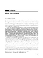
Example The JK flip-flop of Figure 5.3 will be used to illustrate the cut process.
First, according to step 1, an intrinsic weight is assigned to each net. (Each net num-
ber is identified with the number of the gate or primary input that drives it.)
Figure 5.3 Cutting Loops.
1 2 3 4 5 6 7 8 9 10 11 12 13 14
2020210011 0 0 1 1
Q
Clear
Preset
Clock
Q

J
K
1
2
3
4
5
6
7
8
9
10
11
12
13
14
244
SEQUENTIAL LOGIC TEST
Next, assign weights:
From step 2 it is determined that line 6 must be assigned a weight of 3. At this point
no other line can be assigned. The unweighted successors of the weighted lines con-
sists of the set
A = {7,8,9,10,11,12,13,14}
A net is chosen and its SCC is determined. If net 7 is arbitrarily chosen, we find that
its SCC is the entire set A. Since the SCC is the only loop in the circuit, all predeces-
sors of the SCC are weighted so processing of the SCC can proceed.
We compute the periods of the nets in the SCC and find that nets 9, 10, 13, and 14
have period 2. Therefore, B = {9, 10, 13, 14}. In the set A
−
B = {7, 8, 11, 12} all

nets have at least one weighted predecessor, so U = A
−
B. It also turns out that
U
1
= U in this case. A net in U
1
is selected that has a predecessor of minimal weight,
say gate 7. A cut is made on net 14 between gate 14 and gate 7. The maximum
weight assigned up to this point was 3. Therefore, we assign a weight of 4 to net 7.
At this point weights cannot be assigned to any additional nets because loops still
exist. The SCC is
A = {8,9,10,11,12,13,14}
The process is repeated, this time a cut is made from gate 13 to gate 8. A weight of 5
is assigned to net 8. This leaves two SCCs, C = {9,10} and D = {13,14}. C must be
chosen because D has unweighted predecessors. A cut is made from 9 to 10. A weight
of 6 is assigned to net 10 and a weight of 2 + 4 + 6 + 1 = 13 to net 9. Weights can now
be assigned to nets 11 and 12. Net 11 is assigned a weight of 13 + 3 + 0 = 16 and net
12 is assigned a weight of 9. Finally, a cut is made from 13 to 14. Net 14 is given the
weight 17 and 13 is given the weight 36. 
The ITG will now be illustrated, using the circuit in Figure 5.4. The original circuit
had one feedback line from the output of J to the input of H that was cut and replaced
by a pseudo-input SI and a pseudo-output SO. The logic gates and primary inputs will
be labeled with letters, and a subscript will be appended to the letters to indicate
which copy of the replicated circuit is being referred to during the discussion.
We assume a SA1 fault on the output of gate E. A test for that fault requires a D
on the net; so, starting with replica 2, we assign A
2
= 1. The output of E drives gates
F and G, and here the ITG reverts to the sensitized path method, it chooses a single

propagation path based on weights assigned during the cut process. The weights
influence the path selection process: The objective is to try to propagate through the
easiest apparent path. In this instance, the path through gate F
2
is selected. It
requires a 0 from D
2
, which in turn requires a 1 on input B
2
. Propagation through K
2
requires a 1 from J
2
and hence 0s on input C
2
and gate H
2
. The 0 on H
2
requires that
1 2 3 4 5 6 7 8 9 10 11 12 13 14
202023
SEQUENTIAL TEST METHODS
245
Figure 5.4 Iterated pseudo-combinational circuit.
pseudo-input SI
2
be a 1. The presence of a non-X value on a pseudo-input must be
justified, so it is necessary to back up to the previous time image.
A 1 on the pseudo-output of J

1
implies 0s on both of its inputs. A 0 from H
1
requires a 1 on one of its inputs. We avoid SI
1
and try to assign G
1
= 1. That requires
E
1
= 0, but E
1
is SA1. We cannot now, in this copy, assume that the output of E
1
is
fault-free. Since it is assumed SA1, we could assign a D, but that places a D and an
X on H
1
, a combination for which there is no entry in the D-algorithm intersection
tables.
The other alternative is to assign a 1 to the pseudo-input, but that is no improve-
ment because the same situation is encountered in the next previous time image. In
practice, a programmed implementation may actually try to justify through the
pseudo-input and go into a potential infinite loop. An implementation must therefore
impose an upper limit on the number of previous time images. If all assignments are
not justified by the time it reaches the limit, it must either give up on that fault or
determine whether an alternative path exists through which to propagate the fault. In
the present case, we can try to propagate through G
2
.

Propagation through G
2
requires B
2
= 0. Then, propagation through H
2
requires a
0 on the pseudo input and propagation through J
2
requires C
2
= 0. Now, however, by
implication F
2
= 0, so it is not possible to propagate through K
2
. Therefore, we
propagate through the pseudo-output SO
2
. The 0 on SI
2
is justified by means of a 0
on J
1
. That is justified by putting a 1 on primary input C
1
.
SO
1
K

1
A
1
B
1
SI
1
C
1
F
1
G
1
H
1
J
1
D
1
E
1
SO
2
K
2
A
2
B
2
SI

2
C
2
F
2
G
2
H
2
J
2
D
2
E
2
SO
3
K
3
A
3
B
3
SI
3
C
3
F
3
G

3
H
3
J
3
D
3
E
3
SA1
D
D
D
D
1
1
0
0
0
D
D
D
D
D
D
D
0
246
SEQUENTIAL LOGIC TEST
A D now appears on the pseudo-input of time image 3. Assigning G

3
= 0 and
C
3
= 0 places a D on the output of J
3
. We set B
3
= 1 to justify the 0 from G
3
and
then try to propagate the D on J
3
through K
3
by assigning F
3
= 1. This requires
D
3
= E
3
= 0. We again find ourselves trying to set the faulted line to a 0. But this
time we set it to D, which causes D to appear on the output of F
3.
Hence both
inputs to K
3
are D and its output is D. The final sequence of inputs is
On the first time image, T

1
inputs A and B have X values. We assign values to
these inputs as per the following rule: If the jth coordinate of the ith pattern is an X,
then set it equal to the value of the jth coordinate on the first pattern number greater
than i for which the jth coordinate has a non-X value. If no pattern greater than i has
a value in the jth coordinate position, assign the most recent preceding value. If the
jth coordinate is never assigned, then set it to the dominant value; that is, if the input
feeds an AND gate set it to 0 and if it feeds an OR gate set it to 1. The objective is to
minimize the number of input changes required for the test and hence minimize or
eliminate races.
The reader may have noted that the cross-coupled NOR latch received input com-
bination (1,1) in time image 1. According to its state table, this is an illegal input
combination. Automatic test pattern generators occasionally assign combinations
that are illegal or illogical when processing sequential circuits. It is one of the rea-
sons why test patterns generated for sequential circuits must be verified through
simulation.
5.3.3 The 9-Value ITG
When creating a test using ITG, it is sometimes the case that more constraints are
imposed than are absolutely necessary. Consider again the circuit of Figure 5.4. We
started by attempting to propagate a test through gate F. That would not work, so we
propagated through G. If we look again at the problem and examine the immediate
effects of propagating a test through gate F, we notice that the faulted circuit,
because it produces a 0 on the upper input when A = B = 1, will produce a 1 on the
output of K regardless of what value occurs on the lower input of K.
The D that was propagated to K implies that the upper input to K will be 1 in
the fault-free circuit. Therefore the output of K for the unfaulted circuit depends
on the value at its lower input. Since we want a sensitized signal on the output of
K, the fault-free circuit must produce a 0 at the circuit output; therefore we want a
1 on the lower input to K.
A 1 can be obtained at the lower input to K by forcing J to produce a 1. This

requires that both inputs to J be 0, which requires the output of H to be 0. Backing
T
1
T
2
T
3
A X1 1
B X0 1
C 100
SEQUENTIAL TEST METHODS
247
up one more step in the logic, we find that H is 0 if either the pseudo-input or G is
1. Gate G cannot be 1 because primary input B is 1. Therefore, a 1 must come
from the pseudo-input. This is the point where we previously failed. The presence
of the fault made it impossible to initialize the cross-coupled latch. Nevertheless,
we will try again. However, this time we ignore the existence of the fault in the
previous copy since we are only concerned with justifying a signal in the good
circuit.
We create a previous time image and attempt to justify a 1 on its pseudo-output.
A 1 can be obtained with C = 0 and G = 1, which requires B = E = 1, and implies
A = 0. Therefore, a successful test is I
1
= (1,0,0) and I
2
= (1,1,0).
In order to distinguish between assignments required for faulted and unfaulted
circuits, a nine-value algebra is used.
4
The definition of the nine values is shown in

Table 5.1. The dashes correspond to unspecified values. The final column shows the
corresponding values for the D-algorithm. It is readily seen that the D-algorithm
symbols are a subset of the nine-value ITG symbols. Tables 5.2 through 5.4 define
the AND, OR, and Invert operations on these signals.
TABLE 5.1 Symbols for Nine-Value ITG
Good Faulted ITG Symbol D Symbol
00 0 0
0X G
0
—
01 S
0
D
X0 F
0
—
XX F
1
—
X1 U X
10 S
1
D
1X G
1
—
11 1 1
TABLE 5.2 AND Operations on Nine Values
0
G

0
S
0
F
0
U
G
1
S
1
F
1
1
0000000000
G
0
0G
0
G
0
0G
0
G
0
0G
0
G
0
S
0

0G
0
S
0
0G
0
G
0
0S
0
S
0
F
0
000F
0
F
0
F
0
F
0
F
0
F
0
U0G
0
G
0

F
0
UUF
0
UU
G
1
0G
0
G
0
F
0
UG
1
S
1
UG
1
S
1
000F
0
F
0
S
1
S
1
S

0
S
1
F
1
0G
0
S
0
F
0
UUS
0
F
1
F
1
10G
0
S
0
F
0
UG
1
S
1
F
1
1

248
SEQUENTIAL LOGIC TEST
To illustrate the use of the tables, we employ the same circuit but start by
assigning S
0
to the output of E
2
in Figure 5.5. The signal is propagated to the upper
input of K
2
, where, due to signal inversions, it becomes S
1
. To propagate an S
1
through the NAND, we check the table for the AND gate. With S
1
on one of its
inputs, a sensitized signal S
1
can be obtained at the output of the AND by placing
either S
1
, G
1
, or a 1 on the other input. The inversion then causes the output of the
NAND to become S
0
. The signal G
1
is the least restrictive of the signals that can be

placed on the other input since it imposes no requirements on the input for the
faulted circuit.
Propagation requires a signal on the other input to F
2
that will not block the sen-
sitized signal. From the table for the OR, we confirm that propagation through F
2
is
Figure 5.5 Test generation with the nine-value ITG.
TABLE 5.3 OR Operations on Nine Values
0
G
0
S
0
F
0
U
G
1
S
1
F
1
1
00G
0
S
0
F

0
UG
1
S
1
F
1
1
G
0
G
0
G
0
S
0
UUG
1
G
1
F
1
1
S
0
S
0
S
0
S

0
F
1
F
1
11F
1
1
F
0
F
0
UF
1
F
0
UG
1
S
1
F
1
1
UUUF
1
UUG
1
G
1
F

1
1
G
1
G
1
G
1
1G
1
G
1
G
1
G
1
11
S
1
S
1
G
1
1S
1
G
1
G
1
S

1
11
F
1
F
1
F
1
F
1
F
1
F
1
11F
1
1
1111111111
TABLE 5.4 Invert Operations On Nine Values
X0G
0
S
0
F
0
UG
1
S
1
F

1
1
Y1G
1
S
1
F
1
UG
0
S
0
F
0
0
SO
1
K
1
A
1
B
1
SI
1
C
1
F
1
G

1
H
1
J
1
D
1
E
1
G
1
G
1
G
1
G
1
G
1
G
0
G
0
G
1
S
0
S
0
S

1
G
0
G
0
X
G
0
G
0
G
1
SO
2
K
2
A
2
B
2
SI
2
C
2
F
2
G
2
G
0

H
2
J
2
D
2
E
2
SA1
SEQUENTIAL TEST METHODS
249
successful with G
0
on the other input. That implies a G
1
on the input of gate
D
2
. Since the input to D
2
is a primary input, the signal is converted to 1. Justi-
fying G
1
from J
2
requires G
0
from each of its inputs. Therefore, we need a G
0
from gate H

2
, which implies a 1 at an input to H
2
. The output of G
2
is 0 so the
value G
1
must be obtained from the pseudo-input. We create a previous time
image and require a G
1
from J
1
. We then need G
0
from primary input C and
also from H
1
. That implies a G
1
from one of the inputs to H
1
, which implies G
0
on both inputs to gate G
1
. A G
0
from inverter E
1

is obtained by placing a G
1
on
its input.
When justifying assignments, different values may be required on different paths
emanating from a gate with fanout. These may or may not conflict, depending on the
values required along the two paths. If one path requires G
1
and the other requires
S
1
, then both requirements can be satisfied with signal S
1
. If one path requires G
1
and the other requires S
0
, then there is a conflict because G
1
requires that the
unfaulted circuit produce a logic 1 at the net and S
0
requires that the unfaulted cir-
cuit produce a logic 0.
5.3.4 The Critical Path
We have seen that, when attempting to develop a test for a sequential circuit, it
is often not possible to reach a primary output in the present time frame (cf.
Figure 5.2); fault effects must be propagated through flip-flops, into the next
time image. But, when entering the next time frame, propagating the fault effect
forward may require additional values from the previous time frame. Hence, it

may become necessary to back up into the previous time frame in order to sat-
isfy those additional values. This process of propagating, and then backing up
into previous time frames, may occur repeatedly if a fault effect requires propa-
gation through several future time frames. Resolving conflicts across time
frames becomes a major problem. The critical path method described in Chap-
ter 4 has sequential as well as combinational circuit processing capability.
Because it always starts at a primary output and works back in time, it avoids
this problem.
Its operation on a sequential circuit is described by means of an example, using
the JK flip-flop of Figure 5.3. Recall that the critical path begins by assigning a
value to an output. It then works its way back toward the input pins, creating a criti-
cal path along the way. Therefore, we start by assigning a 0 to the output of gate 13.
This puts critical 1s on the inputs of gate 13, any one of which failing to the opposite
state will cause an erroneous output.
Gate 11 is then selected. A 0 is assigned to gate 6 to force a 1 from gate 11. To
make it critical we assign a 1 to gate 9. The assignment of a 0 to gate 6 forces assign-
ment of 1s to input 3 and gate 12. Gate 14 is selected next. Since gate 13 is a 0 and
gate 12 is a 1, we can create a critical 0 by assigning a 1 to input 5. The presence of
a 0 on gate 13 also implies a 1 on the output of gate 8; hence gate 10 has a 0 on its
output. To ensure that gate 9 has a 1, a 0 is assigned to gate 7. That in turn requires
input 1 be assigned a 1.
250
SEQUENTIAL LOGIC TEST
Notice that the loop consisting of {13,14} has 1s on all predecessor inputs while
the loop {9,10} is forced to its state by the 0 on gate 7. Since the inputs to loop
{13,14} cannot force it to its state, the loop must be initialized to its state by a previ-
ous pattern. Therefore, the loop {13,14} becomes the initial objective of a preceding
pattern. An assignment of 0 to input 5 and a 1 to inputs 1 and 3 forces the latch to the
correct state.
One additional operation is performed here. The Clear input to gate 14 is made

critical by reversing the values on the loop {13,14} in a previous third time image.
The Preset is set to 0 and the Clear is set to 1. The complete input sequence then
becomes
The pattern at time T
1
resets the latch {13,14}. The pattern at time T
2
sets the latch;
hence the 0 on input 5 at time T
2
is critical. Then, at time T
3
, there is a critical path
from input 3, through gates 6, 11, and 13. A failure on that path will cause the latch
{13,14} to switch to the opposite state.
5.3.5 Extended Backtrace
The critical path is basically a justification operation, since its starting point is a
primary output. Operating in this manner, it completely avoids the propagation
operation, as well as the justification operations that may occur at each time-
frame boundary. The extended backtrace (EBT)
5
bears some resemblance to the
critical path. However, before backing up from a primary output, it selects a
fault. Then, from that fault, a topological path (TP) is traced forward to an out-
put. The TP may pass through sequential elements, indicating that several time
frames are required to propagate the fault effect to an observable output. Along
the way, other sequential subcircuits may need to be set up. This is illustrated in
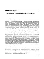
Figure 5.6.
In this hypothetical circuit, assume that the state machine has eight states and that
input I controls the state transitions. Assume that net L

2
= 1 when in state S
8
, L
3
= 1
when in state S
7
, and L
7
= 1 when in S
6
. Otherwise L
2
, L
3
, and L
7
equal 0. The com-
parator contains a counter, denoted B, and when the value in B equals the value on
the A input port, net L
1
= 0, otherwise L
1
= 1. The goal is to create a test for the SA1
fault on net L
1
.
One approach to solving this goal might be to begin by justifying the condition
A = B at the comparator. Once a match is obtained, the next clock pulse causes the

T
1
T
2
T
3
1011
2XX1
3111
4XXX
5101
SEQUENTIAL TEST METHODS
251
Figure 5.6 Aligning Sequential Circuits.
value 0 on L
1
to propagate through the flip-flop and reach AND gate F. To propagate
through F it is necessary for nets L
2
and L
6
to be justified to 1. Should they be pro-
cessed individually, or should they be processed in parallel? And should the vectors
generated when processing L
2
and L
6
be positioned in the vector stream prior to, or
after, those generated while justifying the comparator? The problem is complicated
by the fact that L

6
not only depends on E, but also requires the state machine to tran-
sition through states S
6
and S
7
, whereas L
2
requires the state machine to be in state
S
8
. The human observer can see that these are sequentially solvable, but the com-
puter lacks intuition.
EBT begins by creating a TP to the output. The TP includes L
1
, F, and Z.
From the output Z, the requirement L
5
, L
2
, L
6
= (0,1,1) is imposed. This consti-
tutes a current time frame (CTF) solution or vector. This CTF will often require
a previous time frame (PTF) vector. The PTF is the complete set of assignments
to flip-flops and primary inputs that satisfy the requirements for the CTF. Essen-
tially, EBT is backing up along all paths in parallel, but with the proviso that the
fault effect must propagate along the TP. Eventually, the goal is to reach a vector
that does not rely on a PTF. At that point a self-initializing sequence exists that
can test the fault. This last vector that is created is the first to be applied to the

circuit.
EBT is simplified by the fact that forward propagation software is not required.
However, the TP imposes requirements as it is traced forward, so during backtrace
the TP requirements must be added to the requirements encountered during back-
trace in order for the fault to become sensitized and eventually propagate forward to
an output. Another advantage to EBT is the fact that vectors do not need to be
inserted between vectors already created. Since processing always works backwards
QD
CLK
QD
A = B
Comparator
I
A
load
State
Machine
L
1
L
2
clear
Q
D
L
4
E
L
6
L

5
En
L
3
Z
F
L
7
En