Computer Applications in Bioprocessing

Advances in Biochemical Engineering/
Biotechnology,Vol. 70
Managing Editor: Th. Scheper
© Springer-Verlag Berlin Heidelberg 2000
Computer Applications in Bioprocessing
Henry R. Bungay
Howard P. Isermann, Department of Chemical Engineering, Rensselaer Polytechnic Institute,
Troy, NY 12180-3590, USA
E-mail:
Biotechnologists have stayed at the forefront for practical applications for computing. As
hardware and software for computing have evolved, the latest advances have found eager
users in the area of bioprocessing. Accomplishments and their significance can be ap-
preciated by tracing the history and the interplay between the computing tools and the
problems that have been solved in bioprocessing.
Keywords.
Computers, Bioprocessing, Artificial intelligence, Control, Models, Education.
1Introduction . . . . . . . . . . . . . . . . . . . . . . . . . . . . . . . 110
2 Historical Development . . . . . . . . . . . . . . . . . . . . . . . . . 111
3Biotechnology . . . . . . . . . . . . . . . . . . . . . . . . . . . . . . 117
3.1 Simulation . . . . . . . . . . . . . . . . . . . . . . . . . . . . . . . . 117
3.2 Monitoring and Control of Bioprocesses . . . . . . . . . . . . . . . . 119
3.3 Bioprocess Analysis and Design . . . . . . . . . . . . . . . . . . . . 120
4 Recent Activities . . . . . . . . . . . . . . . . . . . . . . . . . . . . . 120
4.1 Models . . . . . . . . . . . . . . . . . . . . . . . . . . . . . . . . . . . 120
4.1.1 Unstructured Models . . . . . . . . . . . . . . . . . . . . . . . . . . 121
4.1.2 Structured Models . . . . . . . . . . . . . . . . . . . . . . . . . . . . 121
4.2 Bioprocess Control and Automation . . . . . . . . . . . . . . . . . . 122
4.2.1 Sensors . . . . . . . . . . . . . . . . . . . . . . . . . . . . . . . . . . 123
4.2.2 Observers . . . . . . . . . . . . . . . . . . . . . . . . . . . . . . . . . 123
4.2.3 Auxostats . . . . . . . . . . . . . . . . . . . . . . . . . . . . . . . . . 124
4.2.4 Examples . . . . . . . . . . . . . . . . . . . . . . . . . . . . . . . . . 124

4.2.5 Modeling and Control of Downstream Processing . . . . . . . . . . 125
4.3 Intelligent Systems . . . . . . . . . . . . . . . . . . . . . . . . . . . . 126
4.3.1 Expert Systems . . . . . . . . . . . . . . . . . . . . . . . . . . . . . . 127
4.3.2 Fuzzy Logic . . . . . . . . . . . . . . . . . . . . . . . . . . . . . . . . 127
4.3.3 Neural Networks . . . . . . . . . . . . . . . . . . . . . . . . . . . . . 128
4.4 Responses of Microbial Process . . . . . . . . . . . . . . . . . . . . . 129
4.5 Metabolic Engineering . . . . . . . . . . . . . . . . . . . . . . . . . . 130
5 Information Management . . . . . . . . . . . . . . . . . . . . . . . . 130
5.1 Customer Service . . . . . . . . . . . . . . . . . . . . . . . . . . . . . 131
5.2 Electronic Communication and Teaching with Computers . . . . . 131
6 Some Personal Tips . . . . . . . . . . . . . . . . . . . . . . . . . . . 133
7 Conclusions and Predictions . . . . . . . . . . . . . . . . . . . . . . 134
Appendix: Terminology for Process Dynamics and Control . . . . . . . . 135
References . . . . . . . . . . . . . . . . . . . . . . . . . . . . . . . . . . . . 137
1
Introduction
To provide some historical perspective about what people were doing with
computers and what has changed, I will follow the personalized approach used
by others [1]. While pursuing my B. Chem. Eng. and Ph. D. degrees in the late
1940s and early 1950s, I had no contact at all with computers. My thesis was
typewritten with carbon copies. After working for more than 7 years at a large
pharmaceutical firm where the technical people thought that computers were
for payrolls and finance and not of much use for research and development, I
joined the faculty of a university in 1963 where about 20% of the engineering
professors worked with computers. My education in chemical engineering was
not current because my Ph. D. was in biochemistry. I audited a series of five
courses in mathematics, studied process dynamics, helped teach it, and thus
upgraded my engineering skills.
It was obvious that engineers who used computers could compete better in
the real world, so I sought ways to apply computing in both teaching and

research. Some professors still rely on their students for any computing, but I
felt then and continue to think that you cannot appreciate fully what computers
can do when you cannot write programs. I learned FORTRAN but regressed to
BASIC when I began to work mostly with small computers.Along the way I have
written a few Pascal programs and have dabbled with languages such as Forth.
Early in 1997, I switched to Java which presented a very steep learning curve for
me because of its object orientation.
I left teaching for another stint in industry from 1973 until 1976. I was in
management and ordered a minicomputer for my technical staff. I was the
person who used it most but for fairly easy tasks. One program that solved a
production problem was for blending of a selection of input lots of stale blood
to get adequate values of different blood factors in a product used for stan-
dardizing assays in a hospital laboratory. I became fully comfortable with a
minicomputer, but my level of sophistication of programming changed little.
Our only project related to getting computers into manufacturing tried elec-
tronic data logging at the process and carrying the records to the computer for
analysis [2].
By the time I returned to teaching, minicomputers were common. The main-
frame computer was widely used, but we also had rooms full of smart terminals
that were fed their programs from a server. Very soon my research required a
computer in the laboratory because we focused on dynamics and control. For
110
H.R. Bungay
over 20 years we have improved our systems incrementally by upgrading and
extending both our hardware and software. All of my graduate students have
studied process control, and most have used it in their research. Interfacing a
bioreactor to a computer is routine for us, and some of our control algorithms
are quite sophisticated. We make some use of artificial intelligence.
2
Historical Development

When I entered academia, analog computers were important. We think of the
high-speed of digital computers, but analog computers are lightning fast when
handling systems of equations because their components are arranged in
parallel. They integrate by charging a capacitor. With large capacitors, voltages
change slowly, and the output can be sent to a strip chart recorder or X-Y plot-
ter. Small capacitors give rapid changes with the results displayed on an oscil-
loscope. Each coefficient is set with a potentiometer, and the knobs can be
twisted for testing coefficients while watching the graphs change. This used to
be far more convenient than making runs with a digital computer that had
essentially no graphical output; the digital results had to be compared as
columns of numbers on printed pages. Analog computers have about the same
precision as a slide rule, but we are spoiled by the many figures (often in-
significant) provided by a digital computer. The Achilles heel of the analog
computer is the wiring. Each differential equation requires an integrating
circuit; terms in the equation are summed at the integrator’s input. Voltages are
multiplied by constants by using potentiometers. Constants are developed by
taking a fraction of a reference voltage, either plus or minus. With many com-
ponents, jacks for reference voltages, wires going everywhere for intercon-
nections, jacks for inputs and outputs to pots, jacks for initial conditions, and
the like, the hookup for a practical problem resembles a rat’s nest. Furthermore,
a special unit is needed for each multiplication or division, and function
generators handle such things as trig relationships and logarithms. To sum-
marize, analog computers perform summation, integration, and multiplication
by a constant very well but are clumsy for multiplication or division of two
variables and for functional relationships.
Scaling could sometimes be a chore when setting up an analog computer
circuit. The inaccuracy can be great when a constant is not a significant fraction
of a reference voltage. Consider, for example, the constant 0.001 to be developed
from a reference voltage of 10 V. The pot would have to be turned to almost the
end of its range. Proper technique is to scale the constant up at this point and to

scale its effect back down at a later point. In addition to magnitude scaling,
there can be time scaling when rate coefficients are badly matched.
I spent a fair amount of time with analog computers and enjoyed them very
much. I used them for teaching because students could watch graphs change as
they tested permutations of coefficients. One terrible frustration with the
computers that were used for instruction was bad wires. Students, although
admonished not to do so, were thoughtless in yanking wires out of a con-
nection. The wires would come apart inside the plugs where the fault was not
Computer Applications in Bioprocessing
111
visible. Debugging a huge wiring layout and finding out hours later that one or
more of the wires was broken could ruin your day.
I did a little hybrid computing after learning how to do so in a manu-
facturer’s short course. The concept is to let a digital computer control an
analog computer. The example most quoted for using a hybrid computer was
calculations for a space vehicle. The digital computer was better for calculating
the orbit or location and the analog computer, with its parallel and fast inter-
play, was better for calculating pitch, yaw, and roll. The messy wiring and the
difficulty of scaling voltages to match the ranges of the variables doomed both
analog and hybrid computation to near extinction soon after digital computers
had good graphical output.
112
H.R. Bungay
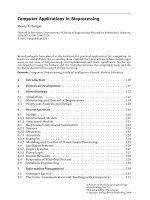
Fig. 1
109 FORMAT (65H FOR SUCH A SHORT TIME, IT IS BEST TO USE A CONTINUOUS
In the early 1960s, FORTRAN was the most popular language for engineers
by far. I learned FORTRAN from books and by examining programs written by
others and began to integrate some digital computing into my courses. There
were several companies that manufactured main frame computers, and
FORTRAN code that I wrote at my university required some modifications

before it could execute on another system when I spent the summer of 1970 at
a different university.
The IBM punch card was used for communicating with the computer. A
typical punched card is shown as Fig. 1. An entire, deep box of cards might be
needed to feed the program and the data into the computer. Typical turn around
time was overnight, and long runs might not be scheduled for two or three days.
Many people were delighted when computer centers could furnish results in an
hour or two. Today we have rooms full of personal computers or work stations.
In the mid 1960s and through the early 1970s there were rooms full of noisy
IBM machines for punching cards. These were fed into a card reader. Wide
paper fed on rolls to the printer ended up fan folded with your results. You
separated pages along the perforations and held them in thick books with metal
strips passed through holes in the paper. There was no graphic output from the
printer except when you devised a way to arrange characters as a crude graph.
To get real graphs you requested a line printer where a pen moved across the
page and touched the paper to make points or lines as the paper was moved
back and forth underneath.
Despite the primitive equipment,much could be done. Libraries of code were
available for various routine tasks such as a least squares fit of an equation to
data points. Remember that the pocket calculator was not common until about
1970 and that mechanical calculators were big, clumsy, noisy, and not very
powerful. Feeding punch cards to a computer seemed the best way to calculate
even when answers were not ready for a few hours.You could get decks of cards
for statistical routines and for various engineering calculations, attach your
data cards, feed the whole pile into a card reader, and return later to the
computer center for your printouts, often far into the night when you were
trying for as many runs as possible. The programs that I wrote were mostly for
numerical solutions of equations. I devised a game that taught my students in
biochemical engineering a little about bioprocess development [3]. The punch
cards had 72 spaces (fields), so I decided upon 7 variables (sugar concentration,

amount of oil, percentage of inoculum, etc.) that each took 10 spaces.
The minicomputer caused a revolution in attitudes. For the first time, the
ordinary user could sit at the computer and work interactively with programs.
Paper tape replaced punch cards, and magnetic storage devices soon took over.
Digital Equipment Corporation sold minicomputers such as their PDP-8 that
was inexpensive enough for a few people to share. There was one just down the
hall from my office, and I could use it for 4 or 5 h each week. Memory was
limited, and programming was at the processor level. You had to code each
operation. For example, multiplication required moving binary numbers in and
out of the central processor, shifting bits, and keeping track of memory
locations. Working with floating point numbers with some bits for the char-
acteristic and others for the mantissa was not easy. You learned to think in
Computer Applications in Bioprocessing
113
binary and then in octal because it was less cumbersome. Before long there were
languages that could simplify operations at an assembly level. Just about the
time I learned one, higher level minicomputer languages appeared soon to be
followed by compilers for real languages such as FORTRAN. Now you could
write code easily, debug interactively, and perform what-if experiments with
your programs. Coils of paper tape for storing programs were superseded by
flat-fold paper tape. Very tough plastic tape was used to some extent.
Minicomputers made it practicable to dedicate a computer to a process.
Groups such as that led by Humphrey at the University of Pennsylvania
developed ways to interface a computer to a bioreactor. Numerous students
wrote new code or improved the code of other students. Much was learned
about sensors, signal conditioning, data display, and process analysis. The
concepts were the bases for commercial software, but the code from the early
days is mostly obsolete. That is not to say that some groups do not still write
code for computer interfacing, but chances are that commercial software will
handle most tasks [4]. Instead of a year or more for writing your own program,

learning to use commercial software takes perhaps 2–6 weeks.
Personal computers intruded on the monopoly of minicomputers, and you
could own a computer instead of sharing with others. The first magnetic storage
that was affordable was an audio tape cassette recorder; the stream of bits from
the computer produced sounds that could be played back and reconverted to
bits. A program might be saved as three or four different files to have high
probability that at least one copy would function properly.
My first personal computer, an Altaire, was build from a kit in 1976 and had
12 kilobytes of memory. A short program had to be toggled in with switches on
the console before the computer could read from a paper tape. You tended to
leave your computer on overnight because mistakes were common when
toggling, and it could be highly annoying to get it booted again. The version of
BASIC that I used took more than 8 kilobytes of the 8-bit memory, leaving little
for the code written by me. One inexpensive way to add memory 4 kilobytes at
a time was to wire a kit for a circuit board, insert memory chips, and plug the
board into the computer.
I must express deep gratitude to students who worked part-time in my
laboratory. We usually had a student from electrical engineering who could
build devices and troubleshoot problems. Today, all of us can be frustrated
when installing new hardware or a new program because the instructions are
not always clear and because following the instructions is no guarantee that the
results will be satisfactory. This is a picnic compared to debugging problems in
the early days. With our home-built computers it was essential to trace circuits,
identify bad chips, and to match cables to the ports. When we had better PCs,
these electrical engineering students were still of great value for constructing
sensor circuits, matching impedances, fixing the A/D converters, connecting
stepping motors, and the like. We built our own preamplifiers for $ 10 worth of
parts, and they performed as well as units costing between $500 and $1000. My
students complained about taking time to construct and test electronic circuits,
but I met students at other universities who complained about equivalent

electronic devices that they purchased. There are delays in shipping and lost
114
H.R. Bungay
time for service with commercial equipment. When something went wrong
with a home-made circuit, we fixed it in a matter of hours instead of waiting for
days or weeks to get outside service. My students learned enough simple
electronics to impress the other graduate students in chemical engineering.
An early input/output device was the teletype. It combined a typewriter,
printer, and paper tape punch/reader. Service with a computer was demanding,
and repairs were frequent. I recall being responsible for three primitive PCs that
were used by students. Each had a teletype, and few weeks went by without lug-
ging one teletype out to my car and going off to get it fixed. Dot matrix printers
made the teletype obsolete. These first printers were noisy, and enclosures to
deaden their sound were popular. Cost of a printer for your PC approached
$1000, and performance was much inferior to units that cost $150 today. I have
owned dot matrix printers, a dot matrix printer with colored ribbons, a laser
printer, and most recently an ink jet color printer that eats up ink cartridges too
quickly.
My next personal computer was similar to the Altaire, but with read-only
memory to get it booted and an eight-inch floppy disk drive. There was some
software for crude word processing. Much of the good software came from
amateurs and was distributed by computer clubs or could be found at uni-
versities. Several years passed before we had graphics capability. I started com-
puting from home by connecting through the phone lines to the university
computer center with a dumb terminal. My wife was taking a course in com-
puting, and we had to drive to the computer center to pick up print outs. Our
modem was so slow that there was hesitation as each character was typed. A dot
matrix printer was soon connected to the spare port on our dumb terminal, and
not so many trips to the computer center were needed. Another computer
purchased for home used our dumb terminal for display and led to mostly local

computing, with the university center available when needed.As faster modems
became available, we upgraded for better service. By about 1982, I was using
electronic communication to colleagues at other institutions. Software was
becoming available for entertainment that provided breaks from serious
programming. My wife became a publisher because my books were integrated
with teaching programs on a disk, and major publishers were leery about
distributing disks and providing customer support for the programs. The
university now had a laser printer that we used to make camera-ready copy for
my books. My wife learned to use some packages for preparing manuscripts
and eventually found that LaTeX was wonderful. The LaTeX commands for
spacing terms in an equation are complicated, and I remember how she spent
hours getting one messy equation to print correctly.
The Apple computer with full color display when connected to a television
set showed what a personal computer could be. Its popularity encouraged com-
petition that brought the price of crude home computers to as low as $100.
Some people in the sciences and in engineering used the Apple computer
professionally, but it was not quite right. It was clumsy for editing text because
letters large enough to read on a TV screen required truncating the line to only
40 characters. You were better off connecting your computer to a monitor with
good, readable, full lines of text. The early IBM computers and the many clones
Computer Applications in Bioprocessing
115
that were soon available had only a monochrome display, but the monitors were
easy to read.
BASIC can do just about anything and is nicely suited to personal computers.
It has ways to get signals from a port and to send signals back. Early FORTRAN
for personal computers did not come with easy ways for reading and writing to
the ports. When most programs were small, it did not matter so much that
BASIC was slow. Its interpretative code runs right away, and FORTRAN and the
other powerful languages require a compiling step.

Interaction with the computer was at the command line at which you typed
your instruction. The graphical user interface was popularized by Apple
Computers and was a sensation with the monochrome Macintosh. While the
Apple company kept close control of its system, IBM used the DOS operating
system that made Bill Gates a billionaire. This was an open system that led to
many companies competing to provide software. Apple has done well in some
niches for software, but PCs that developed from the IBM system have a richer
array of software that has driven them to a predominant share of the market.
I went a different route in the early 1980s with the Commodore Amiga, a
truly magnificent machine that was badly marketed. The Amiga was fast and
great for color graphics because it had specialized chips to assist the central
processor. It had both a command line interface and icons. At one time, I had
five Amiga computers at home, in my office, and in the laboratory. I used the
command line perhaps a little more often than I clicked on an icon.With today’s
Windows, it is not worth the trouble of opening a DOS window so that you can
use a command line and wildcards to make file transfers easy. The Amiga had
true multitasking. This required about 250 kilobytes of memory in contrast to
today’s multitasking systems that gobble memory and require about 80 mega-
bytes of your hard drive. My first Amiga crashed a lot, but later models did not.
My computer purchased in 1998 has the Windows operating system and crashes
two or three times each week.
Minicomputers evolved into workstations and developed side-by-side with
personal computers. Magnetic storage started with large drums or disks and
became smaller in size, larger in capacity, and lower in price. Persistent memory
chips stored programs to get the computer up and running. Eight-inch floppy
disks were rendered obsolete by 5-1/4-inch floppies that gave way to the 3-1/2-
inch disks. The first PCs with hard drives had only 10 megabytes. My first Amiga
with a hard drive (70 megabytes) made dismaying noises as it booted.
Inexpensive personal computers now have options of multi-gigabyte hard
drives. I find essential a Zip drive with 100 megabytes of removable storage.

There are devices with much more removable storage, but I find it easier to keep
track of files when the disk does not hold too many.
It was a logical step to use the ability of the computer as the basis for word
processing. With the early programs, you could only insert and delete on a line-
by-line basis. The next advance was imbedded commands that controlled the
printed page. I was served very well for about seven years by TeX and its off-
shoot LaTeX that had a preview program to show what your pages would look
like. What-you-see-is-what-you-get seems so unremarkable now, but it re-
volutionized word processing. The version of LaTeX for the Amiga came with
116
H.R. Bungay
over a dozen disks with fonts, but there were very few types. These were bit-
mapped fonts, and each size and each style required a different file on the disk.
I obtained fonts at computer shows, bought some Adobe fonts, and found others
in archives at universities. These were intended for PCs, but the files were re-
cognized by my Amiga computer. I had to install them on my hard drive and
learned how to send them to the printer. Proportional fonts that are scaled by
equations have made my a huge collection of bit-mapped fonts obsolete. There
was also incompatibility between PostScript and other printers, but conversion
programs solved this problem.
It may seem extraneous to focus so much on the hardware and software, but
your use of a tool depends on its capabilities. New users today cut their teeth on
word processing, perhaps as part of their e-mail, but this was NOT a common
use of computers in the early days. There were few CRT displays except at the
computer center itself, and users worked with printed pages of output that were
often just long listings of the programs for debugging. These were big pages,
and printing on letter-size paper seems not to have occurred to anyone.
Many of us realized that pictures are better than words and wrote programs
that showed our students not only columns of numbers but also pages with Xs,
Os, and other characters positioned as a graph on the print out. Better graphs

were available from a line printer, but there were few of these, and it was
troublesome to walk some distance to get your results. There was usually a
charge associated with using a line printer, and someone had to make sure that
its pens had ink and were working. There is a great difference between com-
puter output as printed lines of alphanumeric characters and output as
drawings and graphs. It was quite some time before the affordable small
printers for personal computers had graphics capability, but monitors for
graphics became common. Furthermore, the modern computer can update and
animate its images for its CRT display. BASIC for our computers had powerful
graphics calls that were easy to learn. The professional programmers used
languages such as C for high-speed graphics. Programs for word processing
were followed by spreadsheets and other business programs. With the advent of
games, the software industry took off.
3
Biotechnology
Portions of this historical review pertain to academic computing in general, but
there were some specific features for biotechnology. Three interrelated areas of
particular importance are simulation, process monitoring, and process analysis.
3.1
Simulation
Simulation, an important tool for biotechnology, is considered essential by
many bioprocess engineers for designing good control [5]. As you gain under-
standing of a system, you can express relationships as equations. If the solution
of the equations agrees well with information from the real system, you have
Computer Applications in Bioprocessing
117
some confirmation (but not proof) that your understanding has value. Poor
agreement means that there are gaps in your knowledge. Formulating equations
and constructing a model force you to view your system in new ways that
stimulate new ideas.

Modeling of bioprocesses had explosive growth because the interaction of
biology and mathematics excited biochemical engineers. Models addressed
mass transfer, growth and biochemistry, physical chemical equilibria, and
various combinations of each of these.
It becomes impossible to write simple equations when an accumulation of
factors affects time behavior, but we can develop differential equations with
terms for important factors. These equations can be solved simultaneously by
numerical techniques to model behavior in time. In other words, we can reduce
a system to its components and formulate mass balances and rate equations that
integrate to overall behavior.
The concept of a limiting nutrient is essential to understanding biological
processes. The nutrient in short supply relative to the others will be exhausted
first and will thus limit cellular growth. The other ingredients may play various
roles such as exhibiting toxicity or promoting cellular activities, but there will
not be an acute shortage to restrict growth as in the case of the limiting nutrient
becoming exhausted.
The Monod equation deserves special comment. It is but one proposal for
relating specific growth rate coefficient to concentration of growth-limiting
nutrient, but the other proposals seldom see the light of day. This equation is:
m
ˆ
S
m =
01
(1)
Ks + S
where
m = specific growth rate coefficient, time
–1
,

m
ˆ
= maximum specific growth rate, time
–1
,
S = concentration of limiting nutrient, mass/volume, and
Ks = half-saturation coefficient, mass/volume.
Students in biochemical engineering tend to revere the Monod equation, but
practicing engineers apply it with difficulty. There is no time-dependency; it is
not a dynamic relationship and cannot handle sudden changes. Industrial batch
processes encounter variations in the characteristics of the organisms during
the run such that coefficients on the Monod equation must be readjusted.
Simulation paid off. One of my students, Thomas Young, joined Squibb in
about 1970 and soon made major improvements in the yields of two different
antibiotic production batches, mostly as the result of simulation. I had recom-
mended Tom to my old employer. They declined to make him an offer because
they considered him too much of a theoretical type. A vice-president at Squibb
told me that Tom was just about the best person that they ever hired and that
his development research saved their company many millions of dollars. It was
partly the ability to test ideas on the computer that led to rapid progress, but
even more important was the thought process. Deriving equations for simula-
tion forces you to think deeply and analytically, and many new insights arise.
118
H.R. Bungay
3.2
Monitoring and Control of Bioprocesses
Instrumentation in a chemical plant brings to mind the control room of a
petroleum refinery with its walls lined with a cartoon representation of the
processes with dials, charts, controllers, and displays imbedded at the ap-
propriate locations. Operators in the control room observe the data and can

adjust flow rates and conditions. Such control rooms are very expensive but are
still popular.
There are hybrids of the traditional control room with computers for moni-
toring and control. One computer monitor has too little area for displaying all
of a complicated process, and the big boards along the walls may still be
worthwhile. However, smaller processes can be handled nicely on one screen.
Furthermore, a display can go from one process unit to another. A good ex-
ample is the monitoring of a deck that has many bioreactors. One display can
be directed to a selected reactor to show its status, often with graphs showing
variables vs time. The operator can choose the reactor of interest, or each one
can come up for display in sequence. Logic can assign high priority to a reactor
that demands attention so that it is displayed while an alarm sounds or a light
flashes. If we agree that an operator can only watch a relatively small amount of
information anyway, it makes sense to conserve financial resources by omitting
the panel boards and using several computer displays instead. There is the
further advantage that the computer information can be viewed at several loca-
tions; some can be miles away from the factory. Connecting from home can save
a trip to the plant by a technical person at night or at the weekend.
I think that bioprocess companies have done well in using computers to
monitor their processes. The control rooms are full of computers, but the ad-
justments tend to be out in the plant. Only recently have plant operations been
fully automated or converted to control by sending signals from the computers.
Because hardware and the labor to set it up and wire the connections have a
daunting cost, the lifetime of a computerized system is roughly 5 years.
Advances in the technology are so rapid that a system after 5 years is so obsolete
that it is easy to convince management to replace it.
I have an anecdotal report of early attempts at automation. The Commercial
Solvents Corporation in the 1950s attempted to automate sterilization of a
reactor. There was no computer, and the method relied on timers and relays.
Unreliability due to sticky valves and faulty switching resulted in failure. Being

too far ahead of their times gave automation a bad name. Development
engineers at other companies who proposed automation were told that it had
been tried and did not work. Today, there is nothing remarkable about com-
puterized bioreactors and protocols for their operation. I have observed auto-
mated systems in industry that are fully satisfactory. The computer makes up
the medium and can control either batch or continuous sterilization.
Computer Applications in Bioprocessing
119
3.3
Bioprocess Analysis and Design
There is not a great difference now from what was being done in the past, but
there have been many changes in convenience and in capabilities. Engineering
professors wrote programs that assisted process design with such features as
approximating physical properties from thermodynamic equations. These
properties are crucial to such tasks as designing distillation columns but do not
matter much in biochemical engineering. Today, there are excellent commercial
programs such as Aspen that will develop the required thermodynamic
properties en route to designing a process step or even an entire system. I ex-
perimented with Aspen and my opinion of it comes later.
4
Recent Activities
A major advance has been databases and programs that manage databases.
Libraries of genetic sequences have become essential to many biotechnologists,
but this area deserves its own review and will not be mentioned again here.
4.1
Models
Models should be judged on how well they meet some objective. A model that
fails to match a real system can be highly valuable by provoking original ideas
and new departures. Overly complicated computer models, of course, can have
a fatal weakness in the estimation of coefficients. Coefficients measured in

simple systems are seldom valid for complex systems. Often, most of the coef-
ficients in a model represent educated guesses and may be way off. Complicated
models take years to develop and may be impractical to verify. Such models are
worth something because of the organized approach to just about all aspects of
some real system, but there are so many uncertainties and so many opportuni-
ties to overlook significant interactions that predictions based on the models
may be entirely wrong.
Deterministic models (those based on actual mechanisms) make a great deal
of sense when they are not too unwieldy. The terms have physical or biological
meaning and thinking about them may lead to excellent research. The goal of
the modeler should be to identify the most important effects and to eliminate
as many as possible of the insignificant terms. It always comes back to the pur-
pose of modeling. To organize information, we may just keep adding terms to a
model in order to have everything in one place. When the goal is prediction, a
model should be tractable and reliable. That usually means that it must be
simple enough that its coefficients can be estimated and that the model can be
verified by comparing its predictions with known data.
Most real-world situations are too complex for straightforward deterministic
models. Fortunately, there are methods that empirically fit data with mathematical
functions that represent our systems and permit comparisons and predictions.
120
H.R. Bungay