Statistical Description of Data part 2

610
Chapter 14. Statistical Description of Data
Sample page from NUMERICAL RECIPES IN C: THE ART OF SCIENTIFIC COMPUTING (ISBN 0-521-43108-5)
Copyright (C) 1988-1992 by Cambridge University Press.Programs Copyright (C) 1988-1992 by Numerical Recipes Software.
Permission is granted for internet users to make one paper copy for their own personal use. Further reproduction, or any copying of machine-
readable files (including this one) to any servercomputer, is strictly prohibited. To order Numerical Recipes books,diskettes, or CDROMs
visit website or call 1-800-872-7423 (North America only),or send email to (outside North America).
In the other category, model-dependent statistics, we lump the whole subject of
fitting data to a theory, parameter estimation, least-squares fits, and so on. Those
subjects are introduced in Chapter 15.
Section 14.1 deals with so-called measures of central tendency, the moments of
a distribution,the median and mode. In §14.2 we learn to test whether different data
sets are drawn from distributions with different values of these measures of central
tendency. This leads naturally, in §14.3, to the more general question of whether two
distributions can be shown to be (significantly) different.
In §14.4–§14.7, we deal with measures of association for two distributions.
We want to determine whether two variables are “correlated” or “dependent” on
one another. If they are, we want to characterize the degree of correlation in
some simple ways. The distinction between parametric and nonparametric (rank)
methods is emphasized.
Section 14.8 introduces the concept of data smoothing, and discusses the
particular case of Savitzky-Golay smoothing filters.
This chapter draws mathematically on the material on special functions that
was presented in Chapter 6, especially §6.1–§6.4. You may wish, at this point,
to review those sections.
CITED REFERENCES AND FURTHER READING:
Bevington, P.R. 1969,
Data Reduction and Error Analysis for the Physical Sciences
(New York:
McGraw-Hill).
Stuart, A., and Ord, J.K. 1987,

Kendall’s Advanced Theory of Statistics
, 5th ed. (London: Griffin
and Co.) [previous eds. published as Kendall, M., and Stuart, A.,
The Advanced Theory
of Statistics
].
Norusis, M.J. 1982,
SPSS Introductory Guide: Basic Statistics and Operations
; and 1985,
SPSS-
X Advanced Statistics Guide
(New York: McGraw-Hill).
Dunn, O.J., and Clark, V.A. 1974,
Applied Statistics: Analysis of Variance and Regression
(New
York: Wiley).
14.1 Moments of a Distribution: Mean,
Variance, Skewness, and So Forth
When aset of values has a sufficientlystrongcentral tendency, that is, a tendency
to cluster around some particular value, then it may be useful to characterize the
set by a few numbers that are related to its moments, the sums of integer powers
of the values.
Best known is the mean of the values x
1
,...,x
N
,
x=
1
N

N

j=1
x
j
(14.1.1)
which estimates the value around which central clustering occurs. Note the use of
an overbar to denote the mean; angle brackets are an equally common notation,e.g.,
x. You should be aware that the mean is not the only available estimator of this
14.1 Moments of a Distribution: Mean, Variance, Skewness
611
Sample page from NUMERICAL RECIPES IN C: THE ART OF SCIENTIFIC COMPUTING (ISBN 0-521-43108-5)
Copyright (C) 1988-1992 by Cambridge University Press.Programs Copyright (C) 1988-1992 by Numerical Recipes Software.
Permission is granted for internet users to make one paper copy for their own personal use. Further reproduction, or any copying of machine-
readable files (including this one) to any servercomputer, is strictly prohibited. To order Numerical Recipes books,diskettes, or CDROMs
visit website or call 1-800-872-7423 (North America only),or send email to (outside North America).
quantity, nor is it necessarily the best one. For values drawn from a probability
distribution with very broad “tails,” the mean may converge poorly, or not at all, as
the number of sampled points is increased. Alternative estimators, the median and
the mode, are mentioned at the end of this section.
Having characterized a distribution’s central value, one conventionally next
characterizes its “width” or “variability” around that value. Here again, more than
one measure is available. Most common is the variance,
Var ( x
1
...x
N
)=
1
N−1

N

j=1
(x
j
− x)
2
(14.1.2)
or its square root, the standard deviation,
σ(x
1
...x
N
)=

Var(x
1
...x
N
)(14.1.3)
Equation (14.1.2) estimates the mean squared deviation of x from its mean value.
There is a long story about why the denominator of (14.1.2) is N − 1 instead of
N. If you have never heard that story, you may consult any good statistics text.
Here we will be content to note that the N − 1 should be changed to N if you
are ever in the situation of measuring the variance of a distribution whose mean
x is known apriorirather than being estimated from the data. (We might also
comment that if the difference between N and N − 1 ever matters to you, then you
are probably up to no good anyway — e.g., trying to substantiate a questionable
hypothesis with marginal data.)
As the mean depends on the first moment of the data, so do the variance and

standard deviation depend on the second moment. It is not uncommon, in real
life, to be dealing with a distribution whose second moment does not exist (i.e., is
infinite). In this case, the variance or standard deviation is useless as a measure
of the data’s width around its central value: The values obtained from equations
(14.1.2) or (14.1.3) will not converge with increased numbers of points, nor show
any consistency from data set to data set drawn from the same distribution. This can
occur even when the width of the peak looks, by eye, perfectly finite. A more robust
estimatorof the widthisthe average deviation or mean absolutedeviation,definedby
ADev(x
1
...x
N
)=
1
N
N

j=1
|x
j
− x| (14.1.4)
One often substitutes the sample median x
med
for x in equation (14.1.4). For any
fixed sample, the median in fact minimizes the mean absolute deviation.
Statisticians have historically sniffed at the use of (14.1.4) instead of (14.1.2),
since the absolute value brackets in (14.1.4) are “nonanalytic” and make theorem-
proving difficult. In recent years, however, the fashion has changed, and the subject
of robust estimation (meaning, estimation for broad distributions with significant
numbers of “outlier” points) has become a popular and important one. Higher

moments, or statistics involving higher powers of the input data, are almost always
less robust than lower moments or statistics that involve only linear sums or (the
lowest moment of all) counting.
612
Chapter 14. Statistical Description of Data
Sample page from NUMERICAL RECIPES IN C: THE ART OF SCIENTIFIC COMPUTING (ISBN 0-521-43108-5)
Copyright (C) 1988-1992 by Cambridge University Press.Programs Copyright (C) 1988-1992 by Numerical Recipes Software.
Permission is granted for internet users to make one paper copy for their own personal use. Further reproduction, or any copying of machine-
readable files (including this one) to any servercomputer, is strictly prohibited. To order Numerical Recipes books,diskettes, or CDROMs
visit website or call 1-800-872-7423 (North America only),or send email to (outside North America).
(b)(a)
Skewness
negative positive
positive
(leptokurtic)
negative
(platykurtic)


Kurtosis
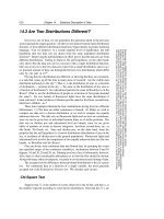
Figure 14.1.1. Distributions whose third and fourth moments are significantly different from a normal
(Gaussian) distribution. (a) Skewness or third moment. (b) Kurtosis or fourth moment.
That being the case, the skewness or third moment,andthekurtosis or fourth
moment should be used with caution or, better yet, not at all.
The skewness characterizes the degree of asymmetry of a distributionaround its
mean. While the mean, standard deviation, and average deviation are dimensional
quantities, that is, have the same units as the measured quantities x
j
, the skewness
is conventionally defined in such a way as to make it nondimensional. It is a pure

number that characterizes only the shape of the distribution. The usual definition is
Skew(x
1
...x
N
)=
1
N
N

j=1

x
j
− x
σ

3
(14.1.5)
where σ = σ(x
1
...x
N
)is the distribution’s standard deviation (14.1.3). A positive
value of skewness signifies a distribution with an asymmetric tail extending out
towards more positive x; a negative value signifies a distribution whose tail extends
out towards more negative x (see Figure 14.1.1).
Of course, any set of N measured values is likely to give a nonzero value
for (14.1.5), even if the underlying distribution is in fact symmetrical (has zero
skewness). For (14.1.5) to be meaningful, we need to have some idea of its

standard deviation as an estimator of the skewness of the underlying distribution.
Unfortunately, that depends on the shape of the underlying distribution, and rather
critically on its tails! For the idealized case of a normal (Gaussian) distribution, the
standarddeviationof (14.1.5) isapproximately

15/N. Inreal lifeitisgoodpractice
to believe in skewnesses only when they are several or many times as large as this.
The kurtosis is also a nondimensional quantity. It measures the relative
peakedness or flatness of a distribution. Relative to what? A normal distribution,
what else! A distribution with positive kurtosis is termed leptokurtic; the outline
of the Matterhorn is an example. A distribution with negative kurtosis is termed
platykurtic; the outline of a loaf of bread is an example. (See Figure 14.1.1.) And,
as you no doubt expect, an in-between distribution is termed mesokurtic.
The conventional definition of the kurtosis is
Kurt(x
1
...x
N
)=



1
N
N

j=1

x
j

− x
σ

4



− 3(14.1.6)
where the −3 term makes the value zero for a normal distribution.
14.1 Moments of a Distribution: Mean, Variance, Skewness
613
Sample page from NUMERICAL RECIPES IN C: THE ART OF SCIENTIFIC COMPUTING (ISBN 0-521-43108-5)
Copyright (C) 1988-1992 by Cambridge University Press.Programs Copyright (C) 1988-1992 by Numerical Recipes Software.
Permission is granted for internet users to make one paper copy for their own personal use. Further reproduction, or any copying of machine-
readable files (including this one) to any servercomputer, is strictly prohibited. To order Numerical Recipes books,diskettes, or CDROMs
visit website or call 1-800-872-7423 (North America only),or send email to (outside North America).
The standard deviation of (14.1.6) as an estimator of the kurtosis of an
underlying normal distribution is

96/N. However, the kurtosis depends on such
a high moment that there are many real-life distributions for which the standard
deviation of (14.1.6) as an estimator is effectively infinite.
Calculation of the quantities defined in this section is perfectly straightforward.
Many textbooks use the binomial theorem to expand out the definitions into sums
of various powers of the data, e.g., the familiar
Var ( x
1
...x
N
)=

1
N−1




N

j=1
x
2
j


− N
x
2


≈
x
2
− x
2
(14.1.7)
but this can magnify the roundoff error by a large factor and is generally unjustifiable
in terms of computing speed. A clever way to minimize roundoff error, especially
for large samples, is to use the corrected two-pass algorithm
[1]
: First calculate x,

then calculate Var(x
1
...x
N
) by
Var(x
1
...x
N
)=
1
N−1





N

j=1
(x
j
− x)
2
−
1
N


N


j=1
(x
j
− x)


2





(14.1.8)
The second sum would be zero if
x were exact, but otherwise it does a good job of
correcting the roundoff error in the first term.
#include <math.h>
void moment(float data[], int n, float *ave, float *adev, float *sdev,
float *var, float *skew, float *curt)
Given an array of
data[1..n]
, this routine returns its mean
ave
, average deviation
adev
,
standard deviation
sdev
,variance

var
,skewness
skew
,andkurtosis
curt
.
{
void nrerror(char error_text[]);
int j;
float ep=0.0,s,p;
if (n <= 1) nrerror("n must be at least 2 in moment");
s=0.0; First pass to get the mean.
for (j=1;j<=n;j++) s += data[j];
*ave=s/n;
*adev=(*var)=(*skew)=(*curt)=0.0; Second pass to get the first (absolute), sec-
ond, third, and fourth moments of the
deviation from the mean.
for (j=1;j<=n;j++) {
*adev += fabs(s=data[j]-(*ave));
ep += s;
*var += (p=s*s);
*skew += (p *= s);
*curt += (p *= s);
}
*adev /= n;
*var=(*var-ep*ep/n)/(n-1); Corrected two-pass formula.
*sdev=sqrt(*var); Put the pieces together according to the con-
ventional definitions.if (*var) {
*skew /= (n*(*var)*(*sdev));
*curt=(*curt)/(n*(*var)*(*var))-3.0;

} else nrerror("No skew/kurtosis when variance = 0 (in moment)");
}
614
Chapter 14. Statistical Description of Data
Sample page from NUMERICAL RECIPES IN C: THE ART OF SCIENTIFIC COMPUTING (ISBN 0-521-43108-5)
Copyright (C) 1988-1992 by Cambridge University Press.Programs Copyright (C) 1988-1992 by Numerical Recipes Software.
Permission is granted for internet users to make one paper copy for their own personal use. Further reproduction, or any copying of machine-
readable files (including this one) to any servercomputer, is strictly prohibited. To order Numerical Recipes books,diskettes, or CDROMs
visit website or call 1-800-872-7423 (North America only),or send email to (outside North America).
Semi-Invariants
The mean and variance of independent random variables are additive: If x and y are
drawn independently from two, possibly different, probability distributions, then
(x + y)=x+y Var(x + y )=Var(x)+Var( x)(14.1.9)
Higher moments are not, in general, additive. However, certain combinations of them,
called semi-invariants, are in fact additive. If the centered moments of a distribution are
denoted M
k
,
M
k
≡

(x
i
− x)
k

(14.1.10)
so that, e.g., M
2

= Var(x), then the first few semi-invariants, denoted I
k
are given by
I
2
= M
2
I
3
= M
3
I
4
= M
4
− 3M
2
2
I
5
= M
5
− 10M
2
M
3
I
6
= M
6

− 15M
2
M
4
− 10M
2
3
+30M
3
2
(14.1.11)
Notice that the skewnessand kurtosis, equations(14.1.5) and (14.1.6) are simple powers
of the semi-invariants,
Skew(x)=I
3
/I
3/2
2
Kurt(x)=I
4
/I
2
2
(14.1.12)
A Gaussian distribution has all its semi-invariants higher than I
2
equal to zero. A Poisson
distribution has all of its semi-invariants equal to its mean. For more details, see
[2]
.

Median and Mode
The median of a probability distribution function p(x) is the value x
med
for
which larger and smaller values of x are equally probable:

x
med
−∞
p(x) dx =
1
2
=

∞
x
med
p(x) dx (14.1.13)
The median of a distribution is estimated from a sample of values x
1
,...,
x
N
by finding that value x
i
which has equal numbers of values above it and below
it. Of course, this is not possible when N is even. In that case it is conventional
to estimate the median as the mean of the unique two central values. If the values
x
j

j =1,...,N are sorted into ascending (or, for that matter, descending) order,
then the formula for the median is
x
med
=

x
(N+1)/2
,Nodd
1
2
(x
N/2
+ x
(N/2)+1
),Neven
(14.1.14)
If a distribution has a strong central tendency, so that most of its area is under
a single peak, then the median is an estimator of the central value. It is a more
robust estimator than the mean is: The median fails as an estimator only if the area
in the tails is large, while the mean fails if the first moment of the tails is large;
it is easy to construct examples where the first moment of the tails is large even
though their area is negligible.
To find the median of a set of values, one can proceed by sorting the set and
then applying (14.1.14). This is a process of order N log N. You might rightly think