Statistical Description of Data part 4
Bạn đang xem bản rút gọn của tài liệu. Xem và tải ngay bản đầy đủ của tài liệu tại đây (209.05 KB, 9 trang )
620
Chapter 14. Statistical Description of Data
Sample page from NUMERICAL RECIPES IN C: THE ART OF SCIENTIFIC COMPUTING (ISBN 0-521-43108-5)
Copyright (C) 1988-1992 by Cambridge University Press.Programs Copyright (C) 1988-1992 by Numerical Recipes Software.
Permission is granted for internet users to make one paper copy for their own personal use. Further reproduction, or any copying of machine-
readable files (including this one) to any servercomputer, is strictly prohibited. To order Numerical Recipes books,diskettes, or CDROMs
visit website or call 1-800-872-7423 (North America only),or send email to (outside North America).
14.3 Are Two Distributions Different?
Given two sets of data, we can generalize the questions asked in the previous
section andask the single question: Arethe two sets drawn from the same distribution
function, or from different distribution functions? Equivalently, in proper statistical
language, “Can we disprove, to a certain required level of significance, the null
hypothesis that two data sets are drawn from the same population distribution
function?” Disprovingthe null hypothesis in effect proves that the data sets are from
different distributions. Failing to disprove the null hypothesis, on the other hand,
only shows that the data sets can be consistent with a single distribution function.
One can never prove that two data sets come from a single distribution, since (e.g.)
no practical amount of data can distinguish between two distributions which differ
only by one part in 10
10
.
Proving that two distributionsare different, or showing that they are consistent,
is a task that comes up all the time in many areas of research: Are the visible stars
distributed uniformly in the sky? (That is, is the distribution of stars as a function
of declination — position in the sky — the same as the distribution of sky area as
a function of declination?) Are educational patterns the same in Brooklyn as in the
Bronx? (That is, are the distributions of people as a function of last-grade-attended
the same?) Do two brands of fluorescent lights have the same distribution of
burn-out times? Is the incidence of chicken pox the same for first-born,second-born,
third-born children, etc.?
These four examples illustrate the four combinations arising from two different
dichotomies: (1) The data are either continuous or binned. (2) Either we wish to
compare one data set to a known distribution, or we wish to compare two equally
unknown data sets. The data sets on fluorescent lights and on stars are continuous,
since we can be given lists of individual burnout times or of stellar positions. The
data sets on chicken pox and educational level are binned, since we are given
tables of numbers of events in discrete categories: first-born, second-born, etc.; or
6th Grade, 7th Grade, etc. Stars and chicken pox, on the other hand, share the
property that the null hypothesis is a known distribution (distribution of area in the
sky, or incidence of chicken pox in the general population). Fluorescent lights and
educational level involve the comparison of two equally unknown data sets (the two
brands, or Brooklyn and the Bronx).
One can always turn continuous data into binned data, by grouping the events
into specified ranges of the continuous variable(s): declinations between 0 and 10
degrees, 10 and 20, 20 and 30, etc. Binning involves a loss of information, however.
Also, there is often considerable arbitrariness as to how the bins should be chosen.
Along with many other investigators,we prefer to avoid unnecessary binning of data.
The accepted test for differences between binned distributions is the chi-square
test. For continuous data as a function of a single variable, the most generally
accepted test is the Kolmogorov-Smirnov test. We consider each in turn.
Chi-Square Test
Suppose that N
i
is the number of events observed in the ith bin, and that n
i
is
the number expected according to some known distribution. Note that the N
i
’s are
14.3 Are Two Distributions Different?
621
Sample page from NUMERICAL RECIPES IN C: THE ART OF SCIENTIFIC COMPUTING (ISBN 0-521-43108-5)
Copyright (C) 1988-1992 by Cambridge University Press.Programs Copyright (C) 1988-1992 by Numerical Recipes Software.
Permission is granted for internet users to make one paper copy for their own personal use. Further reproduction, or any copying of machine-
readable files (including this one) to any servercomputer, is strictly prohibited. To order Numerical Recipes books,diskettes, or CDROMs
visit website or call 1-800-872-7423 (North America only),or send email to (outside North America).
integers, while the n
i
’s may not be. Then the chi-square statistic is
χ
2
=
i
(N
i
− n
i
)
2
n
i
(14.3.1)
where the sum is over all bins. A large value of χ
2
indicates that the null hypothesis
(thatthe N
i
’s aredrawnfromthepopulationrepresented by the n
i
’s) israther unlikely.
Any term j in (14.3.1) with 0=n
j
=N
j
should be omitted from the sum. A
term with n
j
=0,N
j
=0gives an infinite χ
2
, as it should, since in this case the
N
i
’s cannot possibly be drawn from the n
i
’s!
The chi-square probability function Q(χ
2
|ν) is an incomplete gamma function,
and was already discussed in §6.2 (see equation 6.2.18). Strictly speaking Q(χ
2
|ν)
is the probability that the sum of the squares of ν random normal variables of unit
variance (and zero mean) will be greater than χ
2
. The terms in the sum (14.3.1)
are not individually normal. However, if either the number of bins is large ( 1),
or the number of events in each bin is large ( 1), then the chi-square probability
function is a good approximationto the distributionof (14.3.1) in the case of the null
hypothesis. Its use to estimate the significance of the chi-square test is standard.
The appropriate value of ν, the number of degrees of freedom, bears some
additional discussion. If the data are collected with the model n
i
’s fixed — that
is, not later renormalized to fit the total observed number of events ΣN
i
—thenν
equals the number of bins N
B
. (Note that this is not the total number of events!)
Much more commonly, the n
i
’s are normalized after the fact so that their sum equals
the sum of the N
i
’s. In this case the correct value for ν is N
B
− 1, and the model
is said to have one constraint (knstrn=1 in the program below). If the model that
gives the n
i
’s has additional free parameters that were adjusted after the fact to agree
with the data, then each of these additional “fitted” parameters decreases ν (and
increases knstrn) by one additional unit.
We have, then, the following program:
void chsone(float bins[], float ebins[], int nbins, int knstrn, float *df,
float *chsq, float *prob)
Given the array
bins[1..nbins]
containing the observed numbers of events, and an array
ebins[1..nbins]
containing the expected numbers of events, and given the number of con-
straints
knstrn
(normally one), this routine returns (trivially) the number of degrees of freedom
df
, and (nontrivially) the chi-square
chsq
and the significance
prob
. A small value of
prob
indicates a significant difference between the distributions
bins
and
ebins
.Notethat
bins
and
ebins
are both
float
arrays, although
bins
will normally contain integer values.
{
float gammq(float a, float x);
void nrerror(char error_text[]);
int j;
float temp;
*df=nbins-knstrn;
*chsq=0.0;
for (j=1;j<=nbins;j++) {
if (ebins[j] <= 0.0) nrerror("Bad expected number in chsone");
temp=bins[j]-ebins[j];
*chsq += temp*temp/ebins[j];
}
*prob=gammq(0.5*(*df),0.5*(*chsq)); Chi-square probability function. See §6.2.
}
622
Chapter 14. Statistical Description of Data
Sample page from NUMERICAL RECIPES IN C: THE ART OF SCIENTIFIC COMPUTING (ISBN 0-521-43108-5)
Copyright (C) 1988-1992 by Cambridge University Press.Programs Copyright (C) 1988-1992 by Numerical Recipes Software.
Permission is granted for internet users to make one paper copy for their own personal use. Further reproduction, or any copying of machine-
readable files (including this one) to any servercomputer, is strictly prohibited. To order Numerical Recipes books,diskettes, or CDROMs
visit website or call 1-800-872-7423 (North America only),or send email to (outside North America).
Next we consider the case of comparing two binned data sets. Let R
i
be the
number of events in bin i for the first data set, S
i
the number of events in the same
bin i for the second data set. Then the chi-square statistic is
χ
2
=
i
(R
i
− S
i
)
2
R
i
+ S
i
(14.3.2)
Comparing (14.3.2) to (14.3.1), you should note that the denominator of (14.3.2) is
not just the average of R
i
and S
i
(which would be an estimator of n
i
in 14.3.1).
Rather, it is twice the average, the sum. The reason is that each term in a chi-square
sum is supposed to approximate the square of a normally distributed quantity with
unit variance. The variance of the difference of two normal quantities is the sum
of their individual variances, not the average.
If the data were collected in such a way that the sum of the R
i
’s is necessarily
equal to the sum of S
i
’s, then the number of degrees of freedom is equal to one
less than the number of bins, N
B
− 1 (that is, knstrn =1), the usual case. If
this requirement were absent, then the number of degrees of freedom would be N
B
.
Example: A birdwatcher wants to know whether the distribution of sighted birds
as a function of species is the same this year as last. Each bin corresponds to one
species. If the birdwatcher takes his data to be the first 1000 birds that he saw in
each year, then the number of degrees of freedom is N
B
− 1. If he takes his data to
be all the birds he saw on a random sample of days, the same days in each year, then
the number of degrees of freedom is N
B
(knstrn =0). In this latter case, note that
he is also testing whether the birds were more numerous overall in one year or the
other: That is the extra degree of freedom. Of course, any additional constraints on
the data set lower the number of degrees of freedom (i.e., increase knstrn to more
positive values) in accordance with their number.
The program is
void chstwo(float bins1[], float bins2[], int nbins, int knstrn, float *df,
float *chsq, float *prob)
Given the arrays
bins1[1..nbins]
and
bins2[1..nbins]
, containing two sets of binned
data, and given the number of constraints
knstrn
(normally 1 or 0), this routine returns the
number of degrees of freedom
df
, the chi-square
chsq
, and the significance
prob
. A small value
of
prob
indicates a significant difference between the distributions
bins1
and
bins2
.Notethat
bins1
and
bins2
are both
float
arrays, although they will normally contain integer values.
{
float gammq(float a, float x);
int j;
float temp;
*df=nbins-knstrn;
*chsq=0.0;
for (j=1;j<=nbins;j++)
if (bins1[j] == 0.0 && bins2[j] == 0.0)
--(*df); No data means one less degree of free-
dom.else {
temp=bins1[j]-bins2[j];
*chsq += temp*temp/(bins1[j]+bins2[j]);
}
*prob=gammq(0.5*(*df),0.5*(*chsq)); Chi-square probability function. See §6.2.
}
14.3 Are Two Distributions Different?
623
Sample page from NUMERICAL RECIPES IN C: THE ART OF SCIENTIFIC COMPUTING (ISBN 0-521-43108-5)
Copyright (C) 1988-1992 by Cambridge University Press.Programs Copyright (C) 1988-1992 by Numerical Recipes Software.
Permission is granted for internet users to make one paper copy for their own personal use. Further reproduction, or any copying of machine-
readable files (including this one) to any servercomputer, is strictly prohibited. To order Numerical Recipes books,diskettes, or CDROMs
visit website or call 1-800-872-7423 (North America only),or send email to (outside North America).
Equation (14.3.2) and the routine chstwo both apply to the case where the total
number of data points is the same in the two binned sets. For unequal numbers of
data points, the formula analogous to (14.3.2) is
χ
2
=
i
(
S/RR
i
−
R/SS
i
)
2
R
i
+ S
i
(14.3.3)
where
R ≡
i
R
i
S ≡
i
S
i
(14.3.4)
are the respective numbers of data points. It is straightforward to make the
corresponding change in chstwo.
Kolmogorov-Smirnov Test
The Kolmogorov-Smirnov (or K–S) test is applicable to unbinned distributions
that are functions of a single independent variable, that is, to data sets where each
data point can be associated with a single number (lifetime of each lightbulb when
it burns out, or declination of each star). In such cases, the list of data points can
be easily converted to an unbiased estimator S
N
(x) of the cumulative distribution
function of the probability distributionfrom which it was drawn: If the N events are
located at values x
i
,i=1,...,N,thenS
N
(x)is the function giving the fraction
of data points to the left of a given value x. This function is obviously constant
between consecutive (i.e., sorted into ascending order) x
i
’s, and jumps by the same
constant 1/N at each x
i
. (See Figure 14.3.1.)
Different distribution functions, or sets of data, give different cumulative
distribution function estimates by the above procedure. However, all cumulative
distribution functions agree at the smallest allowable value of x (where they are
zero), and at the largest allowable value of x (where they are unity). (The smallest
and largest values might of course be ±∞.) So it is the behavior between the largest
and smallest values that distinguishes distributions.
One can think of any number of statistics to measure the overall difference
between twocumulativedistributionfunctions: theabsolutevalueof thearea between
them, for example. Or their integrated mean square difference. The Kolmogorov-
Smirnov D is a particularly simple measure: It is defined as the maximum value
of the absolute difference between two cumulative distribution functions. Thus,
for comparing one data set’s S
N
(x) to a known cumulative distribution function
P (x), the K–S statistic is
D =max
−∞<x<∞
|S
N
(x) − P (x)| (14.3.5)
while for comparing two different cumulative distribution functions S
N
1
(x) and
S
N
2
(x), the K–S statistic is
D =max
−∞<x<∞
|S
N
1
(x) − S
N
2
(x)| (14.3.6)
624
Chapter 14. Statistical Description of Data
Sample page from NUMERICAL RECIPES IN C: THE ART OF SCIENTIFIC COMPUTING (ISBN 0-521-43108-5)
Copyright (C) 1988-1992 by Cambridge University Press.Programs Copyright (C) 1988-1992 by Numerical Recipes Software.
Permission is granted for internet users to make one paper copy for their own personal use. Further reproduction, or any copying of machine-
readable files (including this one) to any servercomputer, is strictly prohibited. To order Numerical Recipes books,diskettes, or CDROMs
visit website or call 1-800-872-7423 (North America only),or send email to (outside North America).
x
x
D
P( x )
S
N
( x )
cumulative probability distribution
Figure 14.3.1. Kolmogorov-Smirnov statistic D. A measured distribution of values in x (shown
as N dots on the lower abscissa) is to be compared with a theoretical distribution whose cumulative
probability distribution is plotted as P (x). A step-function cumulative probability distribution S
N
(x) is
constructed, one that rises an equal amount at each measured point. D is the greatest distance between
the two cumulative distributions.
What makes the K–S statisticuseful is that its distributionin the case of the null
hypothesis (data sets drawn from the same distribution)can be calculated, at least to
useful approximation, thus giving the significance of any observed nonzero value of
D. A central feature of the K–S test is that it is invariant under reparametrization
of x; in other words, you can locally slide or stretch the x axis in Figure 14.3.1,
and the maximum distance D remains unchanged. For example, you will get the
same significance using x as using log x.
The function that enters into the calculation of the significance can be written
as the following sum:
Q
KS
(λ)=2
∞
j=1
(−1)
j−1
e
−2j
2
λ
2
(14.3.7)
which is a monotonic function with the limiting values
Q
KS
(0) = 1 Q
KS
(∞)=0 (14.3.8)
In terms of this function, the significance level of an observed value of D (as
a disproof of the null hypothesis that the distributions are the same) is given
approximately
[1]
by the formula
Probability (D>observed )=Q
KS
N
e
+0.12 + 0.11/
N
e
D
(14.3.9)