Ten Principles of Economics - Part 47

CHAPTER 21 THE THEORY OF CONSUMER CHOICE 475
INCOME AND SUBSTITUTION EFFECTS
The impact of a change in the price of a good on consumption can be decomposed
into two effects: an income effect and a substitution effect. To see what these two
effects are, consider how our consumer might respond when he learns that the
price of Pepsi has fallen. He might reason in the following ways:
◆ “Great news! Now that Pepsi is cheaper, my income has greater purchasing
power. I am, in effect, richer than I was. Because I am richer, I can buy both
more Pepsi and more pizza.” (This is the income effect.)
◆ “Now that the price of Pepsi has fallen, I get more pints of Pepsi for every
pizza that I give up. Because pizza is now relatively more expensive, I should
buy less pizza and more Pepsi.” (This is the substitution effect.)
Which statement do you find more compelling?
In fact, both of these statements make sense. The decrease in the price of Pepsi
makes the consumer better off. If Pepsi and pizza are both normal goods, the con-
sumer will want to spread this improvement in his purchasing power over both
goods. This income effect tends to make the consumer buy more pizza and more
Pepsi. Yet, at the same time, consumption of Pepsi has become less expensive rela-
tive to consumption of pizza. This substitution effect tends to make the consumer
choose more Pepsi and less pizza.
Now consider the end result of these two effects. The consumer certainly buys
more Pepsi, because the income and substitution effects both act to raise purchases
of Pepsi. But it is ambiguous whether the consumer buys more pizza, because the
Quantity
of Pizza
100
Quantity
of Pepsi
1,000
500
0

B
D
A
New optimum
I
1
I
2
Initial optimum
New budget constraint
Initial
budget
constraint
1. A fall in the price of Pepsi rotates
the budget constraint outward . . .
3. . . . and
raising Pepsi
consumption.
2. . . . reducing pizza consumption . . .
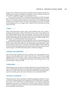
Figure 21-9
AC
HANGE IN
P
RICE
. When the
price of Pepsi falls, the
consumer’s budget constraint
shifts outward and changes
slope. The consumer moves from
the initial optimum to the new

optimum, which changes his
purchases of both Pepsi and
pizza. In this case, the quantity of
Pepsi consumed rises, and the
quantity of pizza consumed falls.
income effect
the change in consumption that
results when a price change moves
the consumer to a higher or lower
indifference curve
substitution effect
the change in consumption that
results when a price change moves
the consumer along a given
indifference curve to a point with a
new marginal rate of substitution
476 PART SEVEN ADVANCED TOPIC
income and substitution effects work in opposite directions. This conclusion is
summarized in Table 21-2.
We can interpret the income and substitution effects using indifference curves.
The income effect is the change in consumption that results from the movement to a higher
indifference curve. The substitution effect is the change in consumption that results from
being at a point on an indifference curve with a different marginal rate of substitution.
Figure 21-10 shows graphically how to decompose the change in the con-
sumer’s decision into the income effect and the substitution effect. When the price
Table 21-2
G
OOD
I
NCOME

E
FFECT
S
UBSTITUTION
E
FFECT
T
OTAL
E
FFECT
Pepsi Consumer is richer, Pepsi is relatively cheaper, so Income and substitution effects act in
so he buys more Pepsi. consumer buys more Pepsi. same direction, so consumer buys
more Pepsi.
Pizza Consumer is richer, Pizza is relatively more Income and substitution effects act in
so he buys more pizza. expensive, so consumer opposite directions, so the total effect
buys less pizza. on pizza consumption is ambiguous.
I
NCOME AND
S
UBSTITUTION
E
FFECTS
W
HEN THE
P
RICE OF
P
EPSI
F
ALLS

Quantity
of Pizza
Quantity
of Pepsi
0
Income
effect
Substitution
effect
B
A
C New optimum
I
1
I
2
Initial optimum
New budget constraint
Initial
budget
constraint
Substitution effect
Income effect
Figure 21-10
I
NCOME AND
S
UBSTITUTION
E
FFECTS

. The effect of a change
in price can be broken down into
an income effect and a substitu-
tion effect. The substitution
effect—the movement along an
indifference curve to a point with
a different marginal rate of
substitution—is shown here as
the change from point A to
point B along indifference
curve I
1
. The income effect—the
shift to a higher indifference
curve—is shown here as the
change from point B on
indifference curve I
1
to point C on
indifference curve I
2
.
CHAPTER 21 THE THEORY OF CONSUMER CHOICE 477
of Pepsi falls, the consumer moves from the initial optimum, point A, to the new
optimum, point C. We can view this change as occurring in two steps. First, the
consumer moves along the initial indifference curve I
1
from point A to point B. The
consumer is equally happy at these two points, but at point B, the marginal rate of
substitution reflects the new relative price. (The dashed line through point B

reflects the new relative price by being parallel to the new budget constraint.)
Next, the consumer shifts to the higher indifference curve I
2
by moving from
point B to point C. Even though point B and point C are on different indiffer-
ence curves, they have the same marginal rate of substitution. That is, the slope
of the indifference curve I
1
at point B equals the slope of the indifference curve I
2
at point C.
Although the consumer never actually chooses point B, this hypothetical point
is useful to clarify the two effects that determine the consumer’s decision. Notice
that the change from point A to point B represents a pure change in the marginal
rate of substitution without any change in the consumer’s welfare. Similarly, the
change from point B to point C represents a pure change in welfare without any
change in the marginal rate of substitution. Thus, the movement from A to B
shows the substitution effect, and the movement from B to C shows the income
effect.
DERIVING THE DEMAND CURVE
We have just seen how changes in the price of a good alter the consumer’s budget
constraint and, therefore, the quantities of the two goods that he chooses to buy.
The demand curve for any good reflects these consumption decisions. Recall that
a demand curve shows the quantity demanded of a good for any given price. We
can view a consumer’s demand curve as a summary of the optimal decisions that
arise from his budget constraint and indifference curves.
For example, Figure 21-11 considers the demand for Pepsi. Panel (a) shows
that when the price of a pint falls from $2 to $1, the consumer’s budget constraint
shifts outward. Because of both income and substitution effects, the consumer in-
creases his purchases of Pepsi from 50 to 150 pints. Panel (b) shows the demand

curve that results from this consumer’s decisions. In this way, the theory of con-
sumer choice provides the theoretical foundation for the consumer’s demand
curve, which we first introduced in Chapter 4.
Although it is comforting to know that the demand curve arises naturally
from the theory of consumer choice, this exercise by itself does not justify devel-
oping the theory. There is no need for a rigorous, analytic framework just to estab-
lish that people respond to changes in prices. The theory of consumer choice is,
however, very useful. As we see in the next section, we can use the theory to delve
more deeply into the determinants of household behavior.
QUICK QUIZ: Draw a budget constraint and indifference curves for Pepsi
and pizza. Show what happens to the budget constraint and the consumer’s
optimum when the price of pizza rises. In your diagram, decompose the
change into an income effect and a substitution effect.
478 PART SEVEN ADVANCED TOPIC
FOUR APPLICATIONS
Now that we have developed the basic theory of consumer choice, let’s use it to
shed light on four questions about how the economy works. These four questions
might at first seem unrelated. But because each question involves household
decisionmaking, we can address it with the model of consumer behavior we have
just developed.
DO ALL DEMAND CURVES SLOPE DOWNWARD?
Normally, when the price of a good rises, people buy less of it. Chapter 4 called
this usual behavior the law of demand. This law is reflected in the downward slope
of the demand curve.
As a matter of economic theory, however, demand curves can sometimes slope
upward. In other words, consumers can sometimes violate the law of demand and
buy more of a good when the price rises. To see how this can happen, consider Fig-
ure 21-12. In this example, the consumer buys two goods—meat and potatoes. Ini-
tially, the consumer’s budget constraint is the line from point A to point B. The
optimum is point C. When the price of potatoes rises, the budget constraint shifts

inward and is now the line from point A to point D. The optimum is now point E.
Quantity
of Pizza
50 1500
50
Demand
(a) The Consumer’s Optimum
Quantity
of Pepsi
0
Price of
Pepsi
$2
1
(b) The Demand Curve for Pepsi
Quantity
of Pepsi
150
B
A
B
A
I
1
I
2
New budget constraint
Initial budget
constraint
Figure 21-11

D
ERIVING THE
D
EMAND
C
URVE
. Panel (a) shows that when the price of Pepsi falls from
$2 to $1, the consumer’s optimum moves from point A to point B, and the quantity of
Pepsi consumed rises from 50 to 150 pints. The demand curve in panel (b) reflects this
relationship between the price and the quantity demanded.
CHAPTER 21 THE THEORY OF CONSUMER CHOICE 479
Notice that a rise in the price of potatoes has led the consumer to buy a larger
quantity of potatoes.
Why is the consumer responding in a seemingly perverse way? The reason is
that potatoes here are a strongly inferior good. When the price of potatoes rises,
the consumer is poorer. The income effect makes the consumer want to buy less
meat and more potatoes. At the same time, because the potatoes have become
more expensive relative to meat, the substitution effect makes the consumer want
to buy more meat and less potatoes. In this particular case, however, the income ef-
fect is so strong that it exceeds the substitution effect. In the end, the consumer re-
sponds to the higher price of potatoes by buying less meat and more potatoes.
Economists use the term Giffen good to describe a good that violates the law
of demand. (The term is named for economist Robert Giffen, who first noted this
possibility.) In this example, potatoes are a Giffen good. Giffen goods are inferior
goods for which the income effect dominates the substitution effect. Therefore,
they have demand curves that slope upward.
Economists disagree about whether any Giffen good has ever been discovered.
Some historians suggest that potatoes were in fact a Giffen good during the Irish
potato famine of the nineteenth century. Potatoes were such a large part of peo-
ple’s diet that when the price of potatoes rose, it had a large income effect. People

responded to their reduced living standard by cutting back on the luxury of meat
and buying more of the staple food of potatoes. Thus, it is argued that a higher
price of potatoes actually raised the quantity of potatoes demanded.
Whether or not this historical account is true, it is safe to say that Giffen goods
are very rare. The theory of consumer choice does allow demand curves to slope
upward. Yet such occurrences are so unusual that the law of demand is as reliable
a law as any in economics.
Quantity
of Meat
A
Quantity of
Potatoes
0
E
C
I
2
I
1
Initial budget constraint
New budget
constraint
D
B
2. . . . which
increases
potato
consumption
if potatoes
are a Giffen

good.
Optimum with low
price of potatoes
Optimum with high
price of potatoes
1. An increase in the price of
potatoes rotates the budget
constraint inward . . .
Figure 21-12
AG
IFFEN
G
OOD
. In this
example, when the price of
potatoes rises, the consumer’s
optimum shifts from point C
to point E. In this case, the
consumer responds to a higher
price of potatoes by buying less
meat and more potatoes.
Giffen good
a good for which an increase in the
price raises the quantity demanded