Pro SQL Server 2008 Analysis Services- P5

CHAPTER 7  BUILDING A CUBE
181
Many-to-Many: If we wanted to define a relationship between customers and products, we would
have to use a many-to-many relationship (one customer can be related to many products; one
product can be related to many customers). To define the relationship, you’ll need to select the
intermediate measure group and then the tables necessary to make the connection.
Data Mining: A relationship necessary for a data-mining dimension. We’ll cover this in more depth
in Chapter 13.

This may all seem like a hassle, but it becomes very important to have this kind of control when we
start looking at more-complex cubes, such as the AdventureWorks cube. A portion of the dimension
usage table from AdventureWorks is shown in Figure 7-15. Note the dimensions that are marked as “no
relation” with various measure groups. For example, the Sales Reasons group is associated with only the
Sales Reason and Internet Sales Order Details dimensions.


Figure 7-15. The dimension usage table for the Adventure Works cube
Having these measure groups and dimensions in a single place can make both development and
maintenance easier, and it also provides end users an ability to combine data in a single report (for
example, Internet Sales vs. Reseller Sales). If these measure groups were in separate cubes, many tools
couldn’t handle mapping to them both. We’ve talked about measure groups a lot. Let’s dig more deeply
into them.
Please purchase PDF Split-Merge on www.verypdf.com to remove this watermark.
CHAPTER 7  BUILDING A CUBE
182
Measures and Measure Groups
We’ve covered the concept of measures quite a few times; measures are the numbers our users are after
to analyze. They’re numbers. In OLAP, they’re generally aggregated in some way so that we can look at
various breakdowns of values. In BIDS, you can find all the measures and measure groups in a cube on
the left side of the Cube Structure tab, as shown in Figure 7-16.

Figure 7-16. The Measures pane in BIDS
Measures
Measures are our numbers. Dimensions are around the edge; measures are in the middle, and where
we’re focused. Measures consist of our transactional data, and the aggregated values as we roll them up
by dimension. A measure generally corresponds to a single column of data in a fact table (the table itself
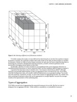
relates to a measure group, covered in a few pages). Take a look at Figure 7-17, showing sales data by
country and territory across the top, and product categories and product lines down the left.

Please purchase PDF Split-Merge on www.verypdf.com to remove this watermark.
CHAPTER 7  BUILDING A CUBE
183

Figure 7-17. Facts and aggregations
Let’s say that our fact data is reported at the territory level by product line—the numbers on a white
background. Those are our facts at the leaf level. They are summed by Analysis Services to produce the
totals by country and by product category (gray background), and the grand totals by country and by
product category (white numbers on a dark gray background). The $10 million figure in the lower right is
the grand total—the summation of every fact in the cube, also the result of the (All) member on every
dimension.
Native measures are generally the result of a single field; however, more-complex measures can be
generated by creating a calculated measure. For example, if a record contains fields for unit cost and
quantity ordered, you could have the subtotal calculated by creating a measure for unit cost × quantity.
You’ll take a closer look at calculated measures later in the chapter.
One of the big things we want from Analysis Services is combining numerical data. Although we
generally think about simply adding the numbers together, there are other ways to combine them.
Selecting a measure in the Measures pane gives us access to the properties for the measure, the first of
which is AggregateFunction. The only truly additive functions (aggregated the same way along every
dimension) are Sum and Count. No matter which way you slice the data, these will return the total (either
adding the values or counting the records) of the child members.

There are two nonadditive aggregations: DistinctCount and None. These do not aggregate numbers.
None simply performs no aggregation—if a combination of dimension members doesn’t return a distinct
value from the fact table, a null is returned. DistinctCount is unique in that its value must be calculated
from the selection of dimension members every time—there aren’t subtotals to “roll up” because
distinct values may collide.
The other aggregate functions are all semiadditive; they can be aggregated along some dimensions,
but not others. As mentioned previously, an inventory measure can be summed along a geographic
dimension (adding inventory stock levels for different locations), but not along the Time dimension (you
can’t take values of 15 widgets in the warehouse in July, 20 widgets in August, and 25 widgets in
September, and add them to get a result of 60 widgets—the value in September should be 25). The
aggregate functions of Min/Max, ByAccount, AverageOfChildren, First/LastChild, and FirstNonEmpty are
all semiadditive aggregation functions.
The DataType property is generally set to Inherited, where it will pick up the data type of the
underlying measure field. You can, however, set it specifically to a data type. The data type must match
the data type of the fact table field, with the exception that if the aggregate function is set to count or
distinct count, the data type will reflect the integer nature of the count value.
Please purchase PDF Split-Merge on www.verypdf.com to remove this watermark.
CHAPTER 7  BUILDING A CUBE
184
DisplayFolder gives you a way to organize measures when you have a large number of them. This is
a free-form text field. Any value you enter here will generate a folder in the measure group with the
measure inside it. Folders with the same name will be combined in a measure group. See Figure 7-18 for
an example.


Figure 7-18. Display folders for organizing measures
If you need to perform a calculation to create the value of the fact data at the leaf level, you can use
MDX in MeasureExpression to be evaluated before any data is aggregated. Consider a quota system in
which selling widgets to customers in certain states gets an additional 10 percent bonus credit for the
salesperson. To calculate the credit correctly, you have to evaluate the sale at the record (that this

specific product was sold to one of those specific customers). Then the values can be added normally.
FormatString is very important . The format code you place here governs how the value is rendered
by client applications (Excel, Reporting Services, and so forth). If you drop down the selector, you can
see preformatted format strings for numeric values, currency, and dates. However, this is a free-form
field, and you can enter any format string by using standard Microsoft formatting conventions.
That sums up the fundamentals of measures. Of course, there’s more we can do with measures—
we’ll look at calculated measures later in the chapter, and KPIs and actions in Chapter 11. We’ll dig into
partitions and aggregations in Chapter 12. For now, let’s take a look at how we deal with groups of
measures.
Measure Groups
A measure group is a collection of measures. (Sorry.) Specifically, they are the OLAP representation of the
underlying fact table that contains the data we’re reporting on. In addition, they also represent the
aggregations that result from rolling up our measure data. A measure group represents all the measures
from a single fact table. The measures within are based on the fields in that table or calculated view in
the data source view. If you create a new measure group (in BIDS, Cube menu
→
New Measure Group),
you’ll be asked which table to base it on. Similarly, if you create a new measure, the New Measure dialog
box will prompt you for a source table and then offer the fields in that table to select from. The table you
select will dictate which measure group will contain the new measure.
As you’ve already seen, measure groups are the containers used to associate dimensions in a cube.
BIDS also uses measure groups as a starting point for partitions and aggregations. By default, partitions
Please purchase PDF Split-Merge on www.verypdf.com to remove this watermark.
CHAPTER 7  BUILDING A CUBE
185
are set by measure group. However, they can be further divided by using a query to split the data in a
measure group (for example, breaking down sales measure data by year). Aggregations are set by
partition, so of course by default they’ll also be set by measure group. We’ll look at partitions and
aggregations later in this chapter.
In general, measure groups are just containers. Let’s take a look at some of the properties of a

measure group and how we can use them, and then we’ll dig into measures themselves. The properties
for a measure group are broken down into the incredibly descriptive groups of Basic, Advanced,
Configurable, Storage, and Misc. Well, let’s not pay any attention to the groupings and just walk through
them:
AggregationPrefix: This property is a leftover from the SQL Server 2000 days, when it was used to set
a prefix on tables created for aggregations. It’s deprecated and will probably be gone in the next
version of SQL Server.
ErrorConfiguration: Here you can set specific responses for errors that occur when processing the
cube. The configuration set here will be used as the error configuration by any new partitions
created for the measure group.
EstimatedRows: You can enter the estimated number of rows per partition here for predictive
calculations. (This number will also be used as the default on new partitions.)
IgnoreUnrelatedDimensions: When this is set to true, any dimensions that are not associated with
the measure group will be forced to the All member when they are included in a query against the
cube. For an unrelated dimension, the measure group will have the same value for every member,
but forcing it back to All makes it clear to the end user what’s happening.
ProcessingMode: Another property that’s actually a default setting for new partitions. In this case,
the options are Regular or LazyAggregations. The Regular setting means that data for the cube won’t
be available for processing until all the aggregations have been calculated. With a setting of
LazyAggregations, users can query the cube after the data is loaded and before all the aggregations
are complete.
Type: Similar to dimension types, there are several options here that help enable special business
intelligence features in Analysis Services.
StorageLocation: This determines where the cache files for the measure group will be stored. If you
click the selector button […] you’ll have a list of locations specified on the server where you can
place the storage files.
DataAggregation: This setting dictates how data can be aggregated for the measure group.
ProactiveCaching: Setting up caching here will set the default proactive caching setting for any
partitions created from the measure group. The dialog should look familiar from when we worked
on proactive caching with dimensions in Chapter 6.

StorageMode: Operates the same as ProactiveCaching, explained in the preceding list item.

One final aspect to measures we want to look at are calculated measures—how we can derive values
from existing values in a fact table.
Calculated Measures
Calculated measures are actually a subset of “calculated dimension members.” However, we want to
focus on calculated measures, because this is where you’ll do most of your calculating.
Please purchase PDF Split-Merge on www.verypdf.com to remove this watermark.
CHAPTER 7  BUILDING A CUBE
186
We’ll start by looking at the Calculations tab of the cube designer, as shown in Figure 7-19. The
organizer is at the top left, calculation tools are in the lower left, and the calculation designer is the right-
hand pane.


Figure 7-19. Designing calculations in our cube
The script organizer lists all the script sections in the current cube. Script sections can be
calculations, named sets, or script commands. There is one script command that is there by default, and
that’s the CALCULATE statement. This is the command that instructs the Analysis Services server to
generate all the aggregations for the cube.

Warning You can end up in an interesting place by accident as a result of the
CALCULATE
statement. If you
create a new calculation and fill in a few fields, and then switch to the script view, you won’t be able to switch
back to the designer, because there will be a syntax error in the script as a result of the unfinished fields. You may
get frustrated and just try a Ctrl+Alt+Delete. The next time you process the cube, it will run fine (no errors), but
you’ll have no aggregated values in your cube (the
CALCULATE
statement didn’t run). The way to fix this is to go

back to the Calculations tab and enter
CALCULATE
for the script command, and then reprocess.
You can create a new calculated member by choosing New Calculated Member from the Cube
menu. This will create a new calculation and open the designer. The calculation will have a default name
Please purchase PDF Split-Merge on www.verypdf.com to remove this watermark.
CHAPTER 7  BUILDING A CUBE
187
and be set to the Measures hierarchy. Note that you also have a Format string, and can set the measure
group and a display folder.
The Expression box seems small, but it will automatically grow as you type. Expressions must be
well-formed MDX. We’ll dig into MDX in depth in Chapter 9, but we’ll look at some lightweight examples
here. Note that the Calculation Tools section in the lower left has the cube structure available. You can
drag and drop measures, dimensions, and hierarchies from here. There’s also a Functions tab, which
lists all the MDX functions you may need (and then some!).
The simplest type of calculated member we’ve referred to previously is figuring out the total for a
line item from the quantity and unit cost. This is some very simple math; we can open the Reseller Sales
folder in the Metadata tab, and drag Order Quantity to the Expression box, type an asterisk (*), and then
drag over Unit Price, which gives us this:

[Measures].[Order Quantity]*[Measures].[Unit Price]

Note that BIDS inserted the parent hierarchy name ([Measures]) for us. So if we name the
calculation [Line Item Total] (standard SQL syntax—you must use square brackets around item names
that have spaces), and set the Format string to Currency, we can process the cube and see results similar
to Figure 7-20.


Figure 7-20. Calculating the line-item total
Hold on, that can’t be right—why are the totals from our calculated measure so much higher than

the total sales amount? Let’s take a look at the order quantity and unit price, shown in Figure 7-21.

Please purchase PDF Split-Merge on www.verypdf.com to remove this watermark.
CHAPTER 7  BUILDING A CUBE
188

Figure 7-21. Adding additional data
If we multiply the Order Quantity shown here by the Unit Price, we can see that it comes out to the
Line Item Total. So it looks like the Line Item Total is being calculated at whatever level we’re at, and that
doesn’t make sense for this type of calculation. (You can’t multiply the total number of items bought for
a period of time by the total of all the Unit Prices—remember we left Unit Price as a sum.) This value
should probably be calculated as a measure expression.
Instead, let’s try calculating the average order amount per sale. We’ll use this formula:

[Measures].[Extended Amount]/[Measures].[Reseller Sales Count]

This type of calculation will work well no matter what type of aggregation we have. In fact, for
averages we actually want to calculate them considering all child data, no matter what level we’re at.
Consider two classrooms, one with 100 students, and the other with 10. The classroom with 100 students
scores an average of 95 percent on an exam, while the classroom with 10 students scores a 75 percent. To
figure the average score across the whole student body, you can’t just average 75 percent and 95 percent
to get 85 percent; you have to go back to the original data and add 110 scores together, and then divide
by 110 (the answer is 93 percent).
And this is a beautiful example of what makes Analysis Services so powerful. When we calculate an
average based on two measures, it will produce the total of the first divided by the total of the second,
based on the measures used and members selected. If we deploy, process, and check the browser, we’ll
see the numbers in Figure 7-22.

Please purchase PDF Split-Merge on www.verypdf.com to remove this watermark.
CHAPTER 7  BUILDING A CUBE

189

Figure 7-22. Calculating average sales amount
We can have more-complex calculations as well. This calculation in the AdventureWorks cube is as
follows:

Case
When IsEmpty( [Measures].[Reseller Sales-Sales Amount] )
Then 0
Else ( [Product].[Product Categories].CurrentMember,
[Measures].[Reseller Sales-Sales Amount]) /
( [Product].[Product Categories].[(All)].[All],
[Measures].[Reseller Sales-Sales Amount] )
End

This will return for any cell associated with a product the ratio of sales for that product (or group of
products) as compared to the sales for all products. You can see what this would look like in Figure 7-23.
Note the CASE statement—if there is no measure from the reseller sales amount, this calculation returns
a zero (for example, if you’re measuring Internet sales). This highlights that calculations run against all
measures in a cube, so if you’re creating a calculation that is specific to a measure, you will need to
exclude it from other measures.
After we’re sure we’re in our Reseller Sales measure, we want to calculate the sales for the currently
selected group against all sales. The first half is an MDX expression indicating to use the currently
selected member, while the second half indicates using all members (the grand total). Note also how the
percentages don’t break down across geography—only across the product hierarchy. However, every
individual product, subcategory, and category is compared to the total.

Please purchase PDF Split-Merge on www.verypdf.com to remove this watermark.
CHAPTER 7  BUILDING A CUBE
190

Figure 7-23. Percentage of sales by product
If we just wanted to see products compared to other products in their subcategory, and
subcategories compared to others in their category, we could simply change the [All] to .Parent. We’ll
dig into MDX more in Chapter 9.
In Exercise 7-2, let’s build a calculated measure just so you can be sure you know what you’re doing.
Exercise 7-2. Create a Calculated Measure
In this exercise, you’ll create a calculated measure in our SSAS AdventureWorks cube and set some
properties to take a look at how it all fits together.
1. Open the SSAS AdventureWorks project if you don’t already have it open.
2. Double-click on the
Adventure Works DW2008.cube
to open it.
3. Click the Calculations tab.
4. From the Cube menu, select New Calculated Member to create a new calculation
and open the designer.
5. Name the calculation [Average Order Amount] (you must include the square
brackets).
6. The Parent hierarchy should already be set to Measures.
7. For the Expression, click the Metadata tab in the Calculation Tools section in the
lower left. Open the measures, then Reseller Sales. Drag Extended Amount to the
Expression window (Figure 7-24).
Please purchase PDF Split-Merge on www.verypdf.com to remove this watermark.
CHAPTER 7  BUILDING A CUBE
191

Figure 7-24. Dragging a field to the Expression box
8. Type a slash (/) after
[Measures].[Extended Amount]
. Then drag Reseller Sales

Count over after the slash. The Expression window should look like Figure 7-25.


Figure 7-25. The calculation expression
9. Change the Format string to $#,##0.00;($#,##0.00).

Tip Don’t use Currency—Excel doesn’t seem to recognize it.
10. Visible should be True, and Associated Measure Group should be Reseller Sales.
11. Open up the Color Expressions section by clicking the two down-arrows next to
the header.
12. Set the Fore Color text to the following:

IIF([Measures].[Average Order Amount]>500, 16711680, 255)
Please purchase PDF Split-Merge on www.verypdf.com to remove this watermark.
CHAPTER 7  BUILDING A CUBE
192
This translates to “If this value is greater than 500, set the text color to blue (16711680); otherwise set it to
red (255).” The numbers are populated if you use the color picker button.
The final Calculation page should look like Figure 7-26.


Figure 7-26. The calculated measure
13. Deploy and process the cube. Then view the measure either in the BIDS browser
or Excel. Both will properly render the formatting and font colors, as shown in
Figure 7-27.
Please purchase PDF Split-Merge on www.verypdf.com to remove this watermark.
CHAPTER 7  BUILDING A CUBE
193

Figure 7-27. Using the calculated measure

14. Save the solution.
Summary
For the most important part of our cubes, it may seem like this went more quickly than the previous
chapter. As I mentioned, generally most of the work is in creating the dimensions. After that’s done,
generating the cube can go fairly quickly. However, we still have more work to do. Although you’ve
deployed things a few times, you really don’t have a strong grasp of what deploy and process really mean.
And that’s what Chapter 8 is about.
Please purchase PDF Split-Merge on www.verypdf.com to remove this watermark.
Please purchase PDF Split-Merge on www.verypdf.com to remove this watermark.
C H A P T E R 8

  

195
Deploying and Processing
We’ve discussed deploying and processing cubes a few times, but it’s been a very rote “push this button,
hope it works” process for you. In this chapter, we’re going to discuss what deploying actually means and
the various ways of doing it. We’ll talk a bit about synchronizing databases between servers—similar to
mirroring for transactional databases. Finally, we’ll talk about processing the various Analysis Services
objects and how to schedule processing should you need to.
Deploying a Project
After you’ve designed an OLAP solution, consisting of data sources, data source views, dimensions, and
cubes, as well as data-mining structures, roles, and assemblies if you created them, you need to deploy
the project to a server before you can actually do anything with it. When you deploy a project, it creates
(or updates) an Analysis Services database. Then all the subordinate objects are created in the database.
Generally, you will deploy a project from BIDS to a development server. If everything passes there,
you can use the Deployment Wizard to deploy the project to testing and production servers. You could
also write code to use Analysis Management Objects (AMO) to manage deployment of SSAS objects. This
becomes particularly compelling when there’s a series of complex operations necessary in deployment,
such as seeding confidential information or connecting a number of disparate systems.

Project Properties
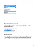
As you saw in earlier exercises, you need to adjust the project properties before you can deploy the
project. If nothing else, you’ll have to change the deployment server name, because the default value is
localhost. To change the project properties, right-click on the solution name and select Properties
(Figure 8-1).

Please purchase PDF Split-Merge on www.verypdf.com to remove this watermark.
CHAPTER 8  DEPLOYING AND PROCESSING
196

Figure 8-1. Opening the project properties
After you have the properties dialog box open (Figure 8-2), you’ll have access to all the properties
that govern deployment of the project to a server. You can choose from multiple configurations by using
the Configuration Manager at the top. Each configuration is simply a collection of settings, so you can
specify which server to deploy to, whether the database should be processed, and so forth.


Figure 8-2. The project properties dialog box
Please purchase PDF Split-Merge on www.verypdf.com to remove this watermark.
CHAPTER 8  DEPLOYING AND PROCESSING
197
Following is a list describing each of the properties available from the dialog box in Figure 8-2. The
list is divided into three parts, one for each tab in the dialog:
Build Tab Properties
• Deployment Server (Edition, Version): Indicates the SSAS edition and version
of the server the database will be deployed to. This will run verifications on
the project you’re trying to deploy to verify all the features you’re trying to use
are in fact available on the target server. For example, perspectives are
available only on the Enterprise Edition of SQL Server Analysis Services. So if
you’re using perspectives and you set the target server edition to Standard,

you will get an error regarding the use of perspectives when you try to deploy.
• Output Path: When you build the solution, a number of structures are
generated (for example, XML manifests). The output path indicates where
these structures should be copied to.
• Remove Passwords: This option will remove any hard-coded passwords from
the data sources you’re using as they’re deployed. If you are hard-coding
passwords, you may not want those stored with the project. Alternatively, you
may work against a development database, but ultimately deploy to test or
production, where you don’t know the passwords and a DBA must go in to
enter these separately (via SSMS).
Debugging Tab Properties
• Start Object: When you start debugging a solution, this is the object that will
be started by BIDS. The Currently Active Object option means that whatever
object is open and has the focus will be where debugging starts. (This is for
debugging .NET stored procedures.)
Deployment Tab Properties
• Processing Option: This option indicates whether BIDS should process the
database after it’s deployed. You may instead choose to deploy a database
solution and have the processing job run during a later maintenance window.
• Transactional Deployment: On occasion you’ll have errors when you process
a database object (we’ll look at this later in the chapter).
• Deployment Mode: The options here are Deploy Changes Only or Deploy
All—simply an option to deploy the full project or just the parts that have
changed. For very large projects, you may want to deploy only the changes,
but deploying the full project ensures that what’s on the server matches what
you’ve been working on.
• Server: This is simply the server name you will deploy to (the default value is
localhost).
• Database: If you need the database to have a different name on the server,
you can change it here. The default value is the name of the project.

Please purchase PDF Split-Merge on www.verypdf.com to remove this watermark.
CHAPTER 8  DEPLOYING AND PROCESSING
198
Deployment Methods
Let’s take a closer look at the methods we have of deploying a database. The methods available include
the following:
AMO Automation: The word automation here is a little bit misleading, considering how much work
we’ve been doing in BIDS to date. The concept here is that you can use AMO to create database
objects on the server. So in theory, you could use code to create dimensions, build cubes, add
members, and so on. Consider a large multinational company that has millions of sales every day—
their sales cubes would be huge. You might set up partitions so that the current quarter’s data is
processed daily, but all historical data is processed only weekly. Instead of setting up new partitions
each quarter, you could have an automated process to move the just-completed quarter’s data into
the current year, and then create a new partition for the current quarter to be processed daily. The
work on the server to make the changes to the database would be effectively considered “deploying”
the new partition.
Backup/Restore: This is an easy way to move a cube intact. If you need a cube available on a system
but would never need to actually process it on the system (perhaps a demo system that doesn’t need
to be absolutely current), then you could back up the cube from the production system and restore
it to the demo system. So long as the source data wasn’t needed again, the cube would function on
the demo system as if it were “live.”
Deployment Wizard: SSAS client tools include a deployment wizard that can be scripted to deploy
databases. When you run the wizard, you’ll be prompted for an Analysis Services database file
(*.asdatabase). You’ll find this in the folder you specified in the project properties. After you’ve
selected the file, walking through the wizard should seem fairly familiar; you’ve seen all the
deployment options before. When you finish the wizard, it will deploy the database and supporting
objects. You will also have the ability to save the deployment as a script that you can run to repeat
the deployment.
Synchronize Database Wizard: This wizard runs similarly to the import/export wizard in SQL
Server. Running the Synchronize Database Wizard copies the cube data and database metadata

from one server to another. This is best used to move databases between development, testing, and
production servers.
XMLA Scripts: Finally, you can deploy a database (or database objects) by generating XML for
Analysis (XMLA) scripts (either from existing objects or by creating your own) and running these
scripts on the server. XMLA scripts can be run from SSMS, an SSIS task, or executed via code.

Now that you have an understanding of the basics of deploying databases in Analysis Services, we’ll
dig a bit into using the Deployment Wizard and synchronizing databases. Then we’ll take a look at
processing databases, cubes, and other database objects.
Using the Deployment Wizard
The SQL Server Analysis Services Deployment Wizard is a stand-alone application. With the Deployment
Wizard, you can take the database file generated when you build an SSAS database from BIDS and either
deploy the database to a target server or generate a deployment script in XMLA.
Please purchase PDF Split-Merge on www.verypdf.com to remove this watermark.
CHAPTER 8  DEPLOYING AND PROCESSING
199
Running the Wizard
The Deployment Wizard is installed with the SQL Server client tools, and can be found via Start
→
All
Programs
→
Microsoft SQL Server 2008
→
Analysis Services. It runs just like a standard wizard; when you
launch it, you’ll get a welcome screen (Figure 8-3).


Figure 8-3. The welcome screen for the Deployment Wizard
As I mentioned earlier, the wizard will ask for the location of the asdatabase file generated by BIDS

when you build an Analysis Services solution. You’ll find this file in the Build location directory
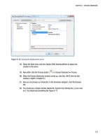
(generally \bin on the project directory). Next you’ll be prompted for the server and database names,
then partition and role options (Figure 8-4). The options for both roles and partitions cover the same
general idea: do you want the deployed database to overwrite or add to existing roles and partitions?

Please purchase PDF Split-Merge on www.verypdf.com to remove this watermark.
CHAPTER 8  DEPLOYING AND PROCESSING
200

Figure 8-4. Role and partition options
The next page of the wizard, shown in Figure 8-5, enables you to specify some key configuration
properties for the objects in the database. On this page, you can edit the connection strings for each data
source, as well as the impersonation information, and indicate the file locations for log files and storage
files.

Please purchase PDF Split-Merge on www.verypdf.com to remove this watermark.