Pro SQL Server 2008 Analysis Services- P6

CHAPTER 9  MDX
231
What if we want a list of the product categories? The first answer is that we can simply list them, as
shown in this query:

SELECT { [Measures].[Reseller Sales Amount] } ON COLUMNS ,
{[Product].[Category].[Accessories],
[Product].[Category].[Bikes],
[Product].[Category].[Clothing],
[Product].[Category].[Components]} ON ROWS
FROM [Adventure Works]

This will return the results shown in Table 9-4. This is fairly straightforward: we’ve selected the
Reseller Sales Amount as our column (header and values), and the set consisting of each category
member from the Category hierarchy in the Product dimension.
Table 9-4. MDX Query Returning Multiple Product Categories
-- Reseller Sales Amount
Accessories $571,297.93
Bikes $66,302,381.56
Clothing $1,777,840.84
Components $11,799,076.66

We’re not restricted to a single column, either. Let’s say we want to compare Reseller Sales Amount
to the cost of freight. We can simply add the Reseller Freight Cost measure to the set we’ve selected for
Columns, as shown next. This produces the result shown in Table 9-5.

SELECT { [Measures].[Reseller Sales Amount],
[Measures].[Reseller Freight Cost]} ON COLUMNS ,
{[Product].[Category].[Accessories],
[Product].[Category].[Bikes],
[Product].[Category].[Clothing],

[Product].[Category].[Components]} ON ROWS
FROM [Adventure Works]
Table 9-5. MDX Query Showing Two Measures as Columns
-- Reseller Sales Amount Reseller Freight Cost
Accessories $571,297.93 $14,282.52
Bikes $66,302,381.56 $1,657,560.05
Clothing $1,777,840.84 $44,446.19
Components $11,799,076.66 $294,977.15
Please purchase PDF Split-Merge on www.verypdf.com to remove this watermark.
CHAPTER 9  MDX
232
Well now we come to an interesting question: how do we use MDX to produce a pivot table? We’ve
done a number of examples showing a breakdown of a value by one dimension in rows, and another
dimension in columns. Can we show Reseller Sales Amount by Categories and Years? Sure we can—or I
wouldn’t have put the question in the book.
Let’s try adjusting the query slightly, as shown next. The results are in Table 9-6.

SELECT { [Date].[Fiscal Year].[FY 2002],
[Date].[Fiscal Year].[FY 2003]} ON COLUMNS ,
{[Product].[Category].[Accessories],
[Product].[Category].[Bikes]} ON ROWS
FROM [Adventure Works]
Table 9-6. MDX Query Using Dimensions for Columns and Rows
-- FY 2002 FY 2003
Accessories $36,814.85 $124,433.35
Bikes $15,018,534.07 $22,417,419.69

We see the selected fiscal years across the column headers—that’s good. And we see the categories
we chose as row headers—also good. But what are those dollar amounts? A little investigation would
show these are the values for the Reseller Sales Amount, but where does that come from? If we check the

cube properties in BIDS, we’ll find that there is a property DefaultMeasure, set to Reseller Sales Amount.
Well that makes sense.
But how do we show a measure other than the Reseller Sales Amount? We can’t add it to either the
ROWS or COLUMNS set, because measures don’t have the same dimensionality as the other tuples in
the set. (See how this is starting to make sense?)
WHERE
What we can do is use a WHERE clause. The WHERE clause in an MDX query works just like the WHERE clause
in a SQL query. It operates to restrict the query’s results. In this case, we can use the WHERE clause to
select what measure we want to return. So we end up with a query as shown here:

SELECT { [Date].[Fiscal Year].[FY 2002],
[Date].[Fiscal Year].[FY 2003]} ON COLUMNS ,
{[Product].[Category].[Accessories],
v[Product].[Category].[Bikes]} ON ROWS
FROM [Adventure Works]
WHERE ([Measures].[Reseller Freight Cost])

In addition to selecting the measure we want to look at, we can also use the WHERE clause to limit
query results in other ways. The following query will show results similar to the previous one, but with
the measure restricted to sales in the United States:

SELECT { [Date].[Fiscal Year].[FY 2002],
[Date].[Fiscal Year].[FY 2003]} ON COLUMNS ,
{[Product].[Category].[Accessories],
Please purchase PDF Split-Merge on www.verypdf.com to remove this watermark.
CHAPTER 9  MDX
233
[Product].[Category].[Bikes]} ON ROWS
FROM [Adventure Works]
WHERE ([Measures].[Reseller Freight Cost],

[Geography].[Country].[United States])

This use of the WHERE clause is also referred to as a slicer, because it slices the cube. When looking at
an MDX query, remember that the WHERE clause is always evaluated first, followed by the remainder of
the query (similar to SQL). Although these two examples seem very different (one selecting a measure,
the other slicing to a specific dimension member), they’re not. Measures in OLAP are just members of
the [Measures] dimension. In that light, both selectors in the second query ([Reseller Freight Cost]
and [United States]) are selecting a single member of their respective dimensions.
Axes
Another way to deal with selecting measures is to simply add another axis, because OLAP is
multidimensional. After all, our “cube” concept started with three dimensions. So why are we limited to
two dimensions (rows and columns) in our query? We’re not. MDX queries can have up to 128 axes, and
the first five are named: COLUMNS, ROWS, PAGES, SECTIONS, CHAPTERS. Beyond those five, then you
simply indicate the axis with an ordinal (for example, ON AXIS 0).
Now, if you try to run an MDX query with three axes in SSMS you’ll get an error; SSMS will tell you
“Results cannot be displayed for cellsets with more than two axes.” In Fast Track to MDX by Mark
Whitehorn, Robert Zare, and Mosha Pasumansky (Springer, 2005), the authors quote ProClarity’s vice-
president of Research and Development regarding ProClarity’s experience with users and more than two
dimensions. The short answer is that flat screens and spreadsheets can show only two dimensions, so
additional dimensions have to be represented in other ways (slicers, pages, and so forth). This can result in
a user getting an initial result that looks incorrect.
Let’s say you want a report of sales by product, by year, and by country. You arrange products in rows,
years in columns, and countries as pages. Now because there are thousands of products, you don’t want
to list them all, especially if most of them will show empty data rows. Well, an MDX query won’t return
products that have no sales data. What gets returned when a specific product has sales in the United
States but not in France? A row will be returned for that product, as it has a sales value. But on the page
for US data, we’ll see the product listed with no values.
The obvious question from a user is “Why is this product listed with no values, but other products I know
exist aren’t listed?” The display gets fairly confusing fairly quickly.
MDX Functions

You saw how to create a grid with multiple member values. However, having to list all the members in a
large hierarchy will get unwieldy very quickly. In addition, if members change, we could end up with
invalidated queries. However, MDX offers functions that we can use to get what we’re looking for. MDX
functions work just as functions in any language: they take parameters and return an object. The return
value can be a scalar value (number), a set, a tuple, or other object.
Please purchase PDF Split-Merge on www.verypdf.com to remove this watermark.
CHAPTER 9  MDX
234
In this case, either the Members function or the Children function will work to give us what we are
looking for. Let’s compare the two. The following query produces the results in Table 9-7.

SELECT { [Measures].[Reseller Sales Amount] } ON COLUMNS ,
{[Product].[Category].Members} ON ROWS
FROM [Adventure Works]
Table 9-7. MDX Query Using Members Function
-- Reseller Sales Amount
All Products $80,450,596.98
Accessories $571,297.93
Bikes $66,302,381.56
Clothing $1,777,840.84
Components $11,799,076.66

Now let’s look at a query using the Children function, and the results shown in Table 9-8.

SELECT { [Measures].[Reseller Sales Amount] } ON COLUMNS ,
{[Product].[Category].Children} ON ROWS
FROM [Adventure Works]
Table 9-8. MDX Query Using Children Function
-- Reseller Sales Amount
Accessories $571,297.93

Bikes $66,302,381.56
Clothing $1,777,840.84
Components $11,799,076.66

It’s pretty easy to see the difference: the Members function returns the All member, while the
Children function doesn’t. If you try this on the [Product Categories] hierarchy, you’ll see the extreme
difference, because Members returns all the members from the [Categories] level, the [Subcategories]
level, and the [Products] level, as shown in Figure 9-7. Note that we have All Products, then Accessories
(category), then Bike Racks (subcategory), and then finally the products in that subcategory. On the
other hand, Figure 9-8 shows selecting all the children under the Mountain Bikes subcategory.

Please purchase PDF Split-Merge on www.verypdf.com to remove this watermark.
CHAPTER 9  MDX
235

Figure 9-7. Selecting a hierarchy Members collection

Figure 9-8. Selecting all the products under the Bikes category
We’ll take a closer look at moving up and down hierarchies later in the chapter.
There’s another difference between SQL and MDX that I haven’t mentioned yet. In SQL we learn
that we cannot depend on the order of the records returned; each record should be considered
independent. However, in the OLAP world result sets are governed by dimensions, and our dimension
members are always in a specific order. This means that concepts such as previous, next, first, and last all
have meaning.
First of all, at any given time in MDX, you have a current member. As we are working with the cube
and the queries, we consider that we are “in” a specific cell or tuple, and so for each dimension we have
a specific member we are working with (or the default member if none are selected).
The CurrentMember function operates on a hierarchy ( [Product Categories] in this case) and
returns a tuple representing the current member. If we run this, we get the result shown in Figure 9-9.
Remember, a tuple is also a set.

Please purchase PDF Split-Merge on www.verypdf.com to remove this watermark.
CHAPTER 9  MDX
236

Figure 9-9. The Reseller Sales Amount query using a CurrentMember function
For example, let’s say for a given cell you want the value from the cell before it (most commonly to
calculate change over time, but you may also want to produce a report of change from one tooling
station to the next, or from one promotion to the next). Generally, the dimension where we have the
most interest in finding the previous or next member is the Time dimension. We frequently want to
compare values for a specific period to the value for the preceding period (in sales there’s even a term for
this—year over year growth).
Let’s look at an MDX query for year over year growth:

WITH
MEMBER [Measures].[YOY Growth] AS
([Date].[Fiscal Quarter].CurrentMember,
[Measures].[Reseller Sales Amount])-
([Date].[Fiscal Quarter].PrevMember,
[Measures].[Reseller Sales Amount])
SELECT NONEMPTY([Date].[Fiscal Quarter].Children *
{[Measures].[Reseller Sales Amount],
[Measures].[YOY Growth]}) ON COLUMNS ,
NONEMPTY([Product].[Model Name].Children) ON ROWS
FROM [Adventure Works]
WHERE ([Geography].[Country].[United States])

There are a number of new features we’re using here. First let’s look at what the results would look
like in the MDX Designer in SSMS, shown in Figure 9-10.

Figure 9-10. Results of the MDX query
Well the first thing we run into is the WITH statement—what’s that? In an MDX query, we use the WITH
statement to define a query-scoped calculated measure. (The alternative is a session-scoped calculated
measure and is defined with the CREATE MEMBER statement, which we won’t cover here.) In this case, we
have created a new measure, [YOY Growth], and defined it.
Please purchase PDF Split-Merge on www.verypdf.com to remove this watermark.
CHAPTER 9  MDX
237
The definition follows the AS keyword, and creates our YOY measure as the difference between two
tuples based on the [Fiscal Quarter] dimension and the [Reseller Sales Amount] measure. In the
tuples, we use the CurrentMember and PrevMember functions. As you might guess, they return the current
member of the hierarchy and the previous member of the hierarchy, respectively.
Look at this statement:

([Date].[Fiscal Quarter].CurrentMember,
[Measures].[Reseller Sales Amount])
-
([Date].[Fiscal Quarter].PrevMember,
[Measures].[Reseller Sales Amount])

Note the two parenthetical operators, which are identical except for the operator at the end. Each
one defines a tuple based on all the current dimension members, except for the [Date] dimension,
where we are taking the current or previous member of the [Fiscal Quarter] hierarchy, and the
[Reseller Sales Amount] member of the [Measures] dimension.
As the calculated measure is used in the query, for each cell calculated, the Analysis Services parser
determines the current member for the hierarchy, and creates the appropriate tuple to find the value of
the cell. Then the previous member is found, and the value for that tuple is identified. Finally, the two
values are subtracted to create the value returned for the specific cell.
Our next new feature in the query is the NONEMPTY function. Consider a query to return all the

Internet sales for customers on July 1, 2001:

SELECT [Measures].[Internet Sales Amount] ON 0,
([Customer].[Customer].[Customer].MEMBERS,
[Date].[Calendar].[Date].&[20010701]) ON 1
FROM [Adventure Works]

If you run this query, you’ll get a list of all 18,485 customers, most of whom didn’t buy anything on
that particular day (and so will have a value of (null) in the cell). Instead, let’s try using NONEMPTY in the
query:

SELECT [Measures].[Internet Sales Amount] ON 0,
NONEMPTY(
[Customer].[Customer].[Customer].MEMBERS,
{([Date].[Calendar].[Date].&[20010701],
[Measures].[Internet Sales Amount])}
) ON 1
FROM [Adventure Works]

The results here are shown in Table 9-9. Note that now we have just the five customers who made
purchases on July 1. The way that NONEMPTY operates is to return all the tuples in a specified set that
aren’t empty. (Okay, that was probably obvious.) Where it becomes more powerful is when you specify
two sets—then NONEMPTY will return the set of tuples from the first set that are empty based on a cross
product with the second set.
Please purchase PDF Split-Merge on www.verypdf.com to remove this watermark.
CHAPTER 9  MDX
238
Table 9-9. Using the NONEMPTY Function
-- Internet Sales Amount
Christy Zhu $8,139.29

Cole A. Watson $4,118.26
Rachael M. Martinez $3,399.99
Ruben Prasad $2,994.09
Sydney S. Wright $4,631.11

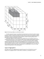
Let’s consider two dimensions, [Geography] and [Parts]. The [Geography] dimension has a
hierarchy including [Region]. Now we want to create a report showing parts purchased by country for
the countries in the North America region (Canada, Mexico, United States). If you look at the data in
Figure 9-11, note that only five of the products out of eleven had sales in the countries we’re interested in
(shaded).


Figure 9-11. Using NONEMPTY
So we want to use the NONEMPTY function:

NONEMPTY(
[Parts].Members,
{
([Geography].[Region].[North America].Members, [Measures].[Sales Amount])
})

Please purchase PDF Split-Merge on www.verypdf.com to remove this watermark.
CHAPTER 9  MDX
239
This will return the list of members of the Parts dimension that have values in the North America
region for the Sales Amount measure, and will evaluate to {[Bike Stands], [Brakes], [Chains],
[Helmets], [Pedals]}.
The second NONEMPTY function has just one argument:

NONEMPTY([Product].[Model Name].Children) ON ROWS

This will evaluate and return a set of members of the Model Name hierarchy that have values in the
current context of the cube (taking into account default members and measures as well as the definition
in the query).
Categories of Functions
Now that you know about functions, it’s time to look at the different categories that are available to you.
MDX offers functions relating to hierarchies, to aggregations, and to time.
Tree Functions
We’ve learned the importance of structure in OLAP dimensions—that’s why we have hierarchies. Now
we’ll get into how to take advantage of those hierarchies in MDX. In SQL we learned to never presume
what order records are in. If we needed a specific order, we had to ensure it in a query or view. In
Analysis Services we define the order in the dimension (or there’s a default order that doesn’t change).
What this means is that we can operate on dimension members to find the next member or previous
member. We can move up to parents or down to children. We do these with a collection of functions that
operate on a member to get the appropriate “relative.” For example, run the following query in SSMS:

SELECT [Measures].[Internet Sales Amount] ON 0,
[Date].[Calendar].[Month].[March 2002].Parent ON 1
FROM [Adventure Works]

This should return the Internet Sales for Q1, Calendar Year 2002, the parent of March 2002 in the
Calendar hierarchy. In the preceding query, Parent is a function that operates on a member and returns
the member above it in the hierarchy. If you execute Parent on the topmost member of a hierarchy, then
SSAS will return a null.
You can “chain” Parent functions—for example, .Parent.Parent to get the “grandparent,” or two
levels up the hierarchy. But this becomes quickly painful. Instead there is the Ancestor() function to
move up a dimensional hierarchy, as shown in the following query.

SELECT [Measures].[Reseller Sales Amount] ON 0,
Ancestor([Product].[Product Categories].[Product].[Chain],

[Product].[Product Categories].[Subcategory]) ON 1
FROM [Adventure Works]

Ancestor() takes two arguments. The first is the dimension member to operate on, and the second
is the hierarchy level to move up to. In the preceding query, we return the Subcategory for the [Chain]
member of products. Ancestor() can also take a numeric value instead of a hierarchy level. In that case,
the result returned is the specified number of steps up from the member in the first argument.
Please purchase PDF Split-Merge on www.verypdf.com to remove this watermark.
CHAPTER 9  MDX
240
■
Note The second argument for
Ancestor()
is the level name, not a member name.
Now that we’ve moved up the tree from a given member, let’s look at how we move down. If you
think about a tree, you should quickly realize that while moving up a tree always gives us a specific
member, moving down a tree is going to give us a collection of members. So it is that while the functions
to move up return members, the functions to move down return sets. If you look at Figure 9-12, the
ancestor of, for example, the Touring Bikes subcategory is the Bikes category (single member). The
ancestor of the Road-150 product is the Road Bikes subcategory (single member). On the other hand, the
descendants of the Bikes category are the Mountain Bikes, Road Bikes, and Touring Bikes subcategories
(set of members).

Figure 9-12. Ancestors vs. descendants in a tree
In the same vein, analogous to the .Parent function, we have .Children. However, as you have
probably figured out, while .Parent returns a member, .Children returns a set. Try the following query:

SELECT [Measures].[Reseller Sales Amount] ON 0,
([Product].[Product Categories].[Bikes].Children) ON 1
FROM [Adventure Works]

Please purchase PDF Split-Merge on www.verypdf.com to remove this watermark.
CHAPTER 9  MDX
241
You should get a breakdown of the reseller sales by the three subcategories under Bikes (Mountain
Bikes, Road Bikes, Touring Bikes).
■
Note If you want to move down a hierarchy but return a single member, you can use the
.FirstChild
or
.LastChild
operators to return a single member from the next level in the hierarchy.
Aggregate Functions
One of the major reasons we’ve wanted to do the OLAP thing is to work with aggregated data. In all the
examples you’ve seen to date, all the individual values are the result of adding the subordinate values
(when we look at sales for Bikes in June 2003, we’re adding all the individual bicycle sales for every
model together for each day in June).
Let’s look at an example:

WITH
MEMBER [Measures].[Avg Sales] AS
AVG({[Product].[Product Categories].CurrentMember.Children},
[Measures].[Reseller Sales Amount])
SELECT
NONEMPTY([Date].[Fiscal Quarter].Children *
{[Measures].[Reseller Sales Amount],
[Measures].[Avg Sales]}) ON COLUMNS ,
NONEMPTY([Product].[Product Categories].Children) ON ROWS
FROM [Adventure Works]
WHERE ([Geography].[Country].[United States])

In this query, we’ve created a calculated measure using the AVG() function, which will average the
value in the second argument across the members indicated in the first argument. In this case we’ve
used CurrentMember to indicate to use the current selected member of the Product Categories hierarchy,
and then take the children of that member. In the SELECT statement, we then use the cross product
between the set of fiscal quarters and the set consisting of the Reseller Sales Amount measure and our
calculated measure. (This produces the output that displays the two measures for each quarter.) Part of
the output is shown in Figure 9-13.


Figure 9-13. The output of the AVG() query
Please purchase PDF Split-Merge on www.verypdf.com to remove this watermark.
CHAPTER 9  MDX
242
We can use Excel to examine the data underlying our grid here. Connect Excel to the
AdventureWorks cube and create a pivot table with Categories down rows, Fiscal Quarters across the
columns, and add a filter for the United States. You can then drill down into the subcategories, as shown
in Figure 9-14, and do the math yourself to check the averages.


Figure 9-14. Verifying the averages from the AVG() query
Another aggregate function that is very useful, and leverages the capabilities of SSAS well, is
TOPCOUNT(). Often when you’re doing analysis on business data, you’ll see the 80/20 rule in action: 80
percent of your sales are in 20 percent of the regions, products, styles, and so forth. So you end up with
charts that look like the one in Figure 9-15.

Please purchase PDF Split-Merge on www.verypdf.com to remove this watermark.
CHAPTER 9  MDX
243

Figure 9-15. Sales across a range of products
What we’re probably interested in is our top performers; for example, how did the top ten products
sell? In T-SQL we can use a TOP function after sorting by the field we’re interested in; in MDX we have
TOPCOUNT().
Let’s adjust our MDX query with the [Avg Sales] measure from before:

WITH
MEMBER [Measures].[Avg Sales] AS
AVG({[Product].[Product Categories].CurrentMember.Children},
[Measures].[Reseller Sales Amount])
SELECT NONEMPTY([Date].[Fiscal Year].Children *
{[Measures].[Reseller Sales Amount],
[Measures].[Avg Sales]}) ON COLUMNS ,
NONEMPTY([Product].[Product Categories].Subcategory.Members) ON ROWS
FROM [Adventure Works]
WHERE ([Geography].[Country].[United States])

First, I’ve changed the time dimension from fiscal quarters to fiscal years, just to make the results
easier to see. Second, I’ve changed the SELECT statement to select Subcategory.Members from the
[Product Categories] hierarchy. Note that I’ve changed .Children to .Members. Although the [Product
Categories] hierarchy has a member named Members, the [Subcategory] level doesn’t, so we use
Children.
Please purchase PDF Split-Merge on www.verypdf.com to remove this watermark.
CHAPTER 9  MDX
244
This query will return results as shown in Figure 9-16. If we just look at FY 2004, the average sales
range from $462 to $362,000. In fact, more than 98 percent of our sales are concentrated in the top ten
items.

Figure 9-16. Results of the Average Sales query across all subcategories
If we want to focus our business on the highest performers, we want to see just those top
performers. So let’s take a look at the query necessary:

WITH
MEMBER [Measures].[Avg Sales] AS
AVG({[Product].[Product Categories].CurrentMember.Children},
[Measures].[Reseller Sales Amount])
SELECT
NONEMPTY([Date].[Fiscal Year].Children *
{[Measures].[Reseller Sales Amount],
[Measures].[Avg Sales]}) ON COLUMNS ,
TOPCOUNT(
[Product].[Product Categories].Subcategory.Members,
10,
[Measures].[Reseller Sales Amount]) ON ROWS
FROM [Adventure Works]
WHERE ([Geography].[Country].[United States])

The only thing I’ve changed here is to add the TOPCOUNT() function to the rows declaration; this will
return the top ten subcategories based on reseller sales. You’ll notice that in several years the top sellers
have a (null) for the sales amount—so why are they in the list? The trick to TOPCOUNT() is that it selects
based on the set as specified for the query. In this case, we get the AdventureWorks cube sliced by the US
geography, and the top subcategories are evaluated from that. After we have those top ten, those
subcategories are listed by fiscal year.
Please purchase PDF Split-Merge on www.verypdf.com to remove this watermark.
CHAPTER 9  MDX
245
Okay, now let’s wrap up our tour of MDX queries with one of the main reasons we really want to use
OLAP: time functions.

Time Functions
Much of the analysis we want to do in OLAP is time based. We want to see how data this month
compares to the previous month, or perhaps to the same month last year (when looking at holiday sales,
you want to compare December to December). Another comparison we often want to make is year to
date, or YTD (if it’s August, we want to compare this year’s performance to the similar period last year,
for example, January to August).
These queries in SQL can run from tricky to downright messy. You end up doing a lot of relative date
math in the SQL language, and will probably end up doing a lot of table scans. In an OLAP solution,
however, we’re simply slicing the cube based on various criteria—what Analysis Services was designed
to do.
So let’s take a look at some of these approaches. We’ll write queries to compare performance from
month to month, to compare a month to the same month the year before, and to compare performance
year to date.
We’ll start with this query:

Select
Nonempty([Date].[Fiscal].[Month].Members) On Columns,
TopCount([Product].[Product Categories].Subcategory.Members,
10,
[Measures].[Reseller Sales Amount]) On Rows
From
[Adventure Works]
Where
([Geography].[Country].[United States], [Date].[Fiscal Year].[FY 2004])

This will give us the reseller sales for the top ten product subcategories for the 12 months in fiscal
2004.
The first thing we want to look at is adding a measure for growth month to month:

WITH

MEMBER [Measures].[Growth] AS
([Date].[Fiscal].CurrentMember,[Measures].[Reseller Sales Amount]) -
([Date].[Fiscal].PrevMember, [Measures].[Reseller Sales Amount])
SELECT NONEMPTY([Date].[Fiscal].[Month].Members
* {[Measures].[Reseller Sales Amount], [Measures].[Growth]})
ON COLUMNS ,
TOPCOUNT([Product].[Product Categories].Subcategory.Members,
10,
[Measures].[Reseller Sales Amount])
ON ROWS
FROM [Adventure Works]
WHERE ([Geography].[Country].[United States], [Date].[Fiscal Year].&[2004])

We’ve added a calculated measure ([Measures].[Growth]) that uses the .CurrentMember and
.PrevMember functions on the [Date].[Fiscal] hierarchy. (Note that you can’t use the member functions
Please purchase PDF Split-Merge on www.verypdf.com to remove this watermark.
CHAPTER 9  MDX
246
on [Date].[Fiscal].[Month], as you may be tempted to—you can use them only on a hierarchy, not a
level.) This will give us a result as shown in Figure 9-17.


Figure 9-17. Showing sales change month to month
Of course, the numbers look awful. Let’s add a FORMAT() statement to our calculated measure:

WITH
MEMBER [Measures].[Growth] AS
Format(([Date].[Fiscal].CurrentMember,
[Measures].[Reseller Sales Amount]) -
([Date].[Fiscal].PrevMember,

[Measures].[Reseller Sales Amount]), "$#,##0.00")

Now we’ll get results that look like Figure 9-18.


Figure 9-18. Formatting our calculated measure
By formatting the measure in the MDX, we find that when we use any well-behaved front end, we
get the same, expected, formatting.
Our bike sales are probably seasonal (mostly sold in the spring and summer, with a spike at
Christmastime), so comparing month to month may not make sense. Let’s take a look at comparing each
month with the same month the previous year. For this, we just need to change our calculated measure
as shown:

WITH
MEMBER [Measures].[Growth] AS
Format(([Date].[Fiscal].CurrentMember,
[Measures].[Reseller Sales Amount]) -
(ParallelPeriod([Date].[Fiscal].[Fiscal Year], 1,
Please purchase PDF Split-Merge on www.verypdf.com to remove this watermark.
CHAPTER 9  MDX
247
[Date].[Fiscal].CurrentMember),
[Measures].[Reseller Sales Amount]), "$#,##0.00")

In this case, we’re using the ParallelPeriod() function. This function is targeted toward time
hierarchies; given a member, a level, and an index, the function will return the corresponding member
that lags by the index count.
■
Note The index in
ParallelPeriod()

is given as a positive integer, but counts backward.
The easiest way to understand this is to look at the illustration in Figure 9-19.


Figure 9-19. Understanding how ParallelPeriod() works
Our final exercise here is to figure out how our revenues compare to last year if it’s August 15. We
can’t compare to last year’s full-year numbers, because that’s comparing eight months of performance
to twelve. Instead, we need last year’s revenues through August 15. First, of course, we need to calculate
the year-to-date sales for our current year. For this we use the PeriodsToDate() function, as shown here:

SUM(PeriodsToDate([Date].[Fiscal].[Fiscal Year],
[Date].[Fiscal].CurrentMember),
[Measures].[Reseller Sales Amount])

The PeriodsToDate() function takes two arguments: a hierarchy level and a member. The function
will return a set of members from the beginning of the period at the level specified up to the member
specified. You can see this is pretty generic; we could get all the days in the current quarter, all the
quarters in the current decade, or whatever.
Please purchase PDF Split-Merge on www.verypdf.com to remove this watermark.
CHAPTER 9  MDX
248
■
Note There is a
YTD()
function in MDX, which is a shortcut for
PeriodsToDate
. The only problem is that it will
work with only calendar years, so here we’re using the more abstract function.
Now let’s calculate the YTD for last year. We’ll do this by using ParallelPeriod() to get the matching
time period last year, and then running the PeriodsToDate() function to return the set of members from

last year up to that member. Here we go:

WITH
MEMBER [Measures].[CurrentYTD] AS
SUM(PeriodsToDate([Date].[Fiscal].[Fiscal Year],
[Date].[Fiscal].CurrentMember),
[Measures].[Reseller Sales Amount])

MEMBER [Measures].[PreviousYTD] AS
SUM(PeriodsToDate([Date].[Fiscal].[Fiscal Year],
ParallelPeriod([Date].[Fiscal].[Fiscal Year],
1,
[Date].[Fiscal].CurrentMember)),
[Measures].[Reseller Sales Amount])

SELECT [Date].[Fiscal].[Month].Members
* {[Measures].[CurrentYTD],
[Measures].[PreviousYTD]}
ON COLUMNS ,
TOPCOUNT([Product].[Product Categories].Subcategory.Members,
10,
[Measures].[Reseller Sales Amount])
ON ROWS
FROM [Adventure Works]
WHERE ([Geography].[Country].[United States],
[Date].[Fiscal Year].&[2004])

This returns the results shown in Figure 9-20.

Figure 9-20. The results of the YTD queries
Please purchase PDF Split-Merge on www.verypdf.com to remove this watermark.
CHAPTER 9  MDX
249
Note that even though I’ve removed the FORMAT() statement, we’ve retained the formatting—an
artifact of summing formatted values. You could still put the statement back if you wanted to ensure
how the numbers would be represented.
Summary
That’s a high-speed tour of MDX, and hopefully now you know enough to be dangerous. Just as T-SQL is
far richer than just the basic SELECT statement, MDX goes much deeper than what we’ve covered here.
My goal was to give you some idea of using MDX against a cube to frame your understanding of MDX in
general. In the next chapter, we’re going to use MDX in some more advanced features of SQL Server
Analysis Services.
Please purchase PDF Split-Merge on www.verypdf.com to remove this watermark.
Please purchase PDF Split-Merge on www.verypdf.com to remove this watermark.