tài liệu cơ sở ngành văn cường ct

Bạn đang xem bản rút gọn của tài liệu. Xem và tải ngay bản đầy đủ của tài liệu tại đây (8.19 MB, 436 trang )

(1)<div class='page_container' data-page=1></div>
(2)<div class='page_container' data-page=2></div>
(3)<div class='page_container' data-page=3></div>
(4)<div class='page_container' data-page=4></div>
(5)<div class='page_container' data-page=5>

MATLAB

®

</div>
(6)<div class='page_container' data-page=6>

MATLAB® For Dummies®

Published by: John Wiley & Sons, Inc., 111 River Street, Hoboken, NJ 07030-5774, www.wiley.com

No part of this publication may be reproduced, stored in a retrieval system or transmitted in any form
or by any means, electronic, mechanical, photocopying, recording, scanning or otherwise, except as
permitted under Sections 107 or 108 of the 1976 United States Copyright Act, without the prior
writ-ten permission of the Publisher. Requests to the Publisher for permission should be addressed to the
Permissions Department, John Wiley & Sons, Inc., 111 River Street, Hoboken, NJ 07030, (201) 748-6011,
fax (201) 748-6008, or online at />

Trademarks: Wiley, For Dummies, the Dummies Man logo, Dummies.com, Making Everything Easier, and
related trade dress are trademarks or registered trademarks of John Wiley & Sons, Inc. and may not be
used without written permission. MATLAB is a registered trademark of Mathworks, Inc. All other
trade-marks are the property of their respective owners. John Wiley & Sons, Inc. is not associated with any
product or vendor mentioned in this book.

LIMIT OF LIABILITY/DISCLAIMER OF WARRANTY: THE PUBLISHER AND THE AUTHOR MAKE NO 
REPRESENTATIONS OR WARRANTIES WITH RESPECT TO THE ACCURACY OR COMPLETENESS OF 
THE CONTENTS OF THIS WORK AND SPECIFICALLY DISCLAIM ALL WARRANTIES, INCLUDING 
WITH-OUT LIMITATION WARRANTIES OF FITNESS FOR A PARTICULAR PURPOSE. NO WARRANTY MAY BE 
CREATED OR EXTENDED BY SALES OR PROMOTIONAL MATERIALS. THE ADVICE AND STRATEGIES 
CONTAINED HEREIN MAY NOT BE SUITABLE FOR EVERY SITUATION. THIS WORK IS SOLD WITH THE 
UNDERSTANDING THAT THE PUBLISHER IS NOT ENGAGED IN RENDERING LEGAL, ACCOUNTING, OR 
OTHER PROFESSIONAL SERVICES. IF PROFESSIONAL ASSISTANCE IS REQUIRED, THE SERVICES OF 
A COMPETENT PROFESSIONAL PERSON SHOULD BE SOUGHT. NEITHER THE PUBLISHER NOR THE 
AUTHOR SHALL BE LIABLE FOR DAMAGES ARISING HEREFROM. THE FACT THAT AN ORGANIZATION

OR WEBSITE IS REFERRED TO IN THIS WORK AS A CITATION AND/OR A POTENTIAL SOURCE OF 
FURTHER INFORMATION DOES NOT MEAN THAT THE AUTHOR OR THE PUBLISHER ENDORSES THE 
INFORMATION THE ORGANIZATION OR WEBSITE MAY PROVIDE OR RECOMMENDATIONS IT MAY 
MAKE. FURTHER, READERS SHOULD BE AWARE THAT INTERNET WEBSITES LISTED IN THIS WORK 
MAY HAVE CHANGED OR DISAPPEARED BETWEEN WHEN THIS WORK WAS WRITTEN AND WHEN 
IT IS READ.

For general information on our other products and services, please contact our Customer Care Department
within the U.S. at 877-762-2974, outside the U.S. at 317-572-3993, or fax 317-572-4002. For technical support,
please visit www.wiley.com/techsupport.

Wiley publishes in a variety of print and electronic formats and by print-on-demand. Some material
included with standard print versions of this book may not be included in e-books or in print-on-demand.
If this book refers to media such as a CD or DVD that is not included in the version you purchased, you
may download this material at . For more information about Wiley
products, visit www.wiley.com.

Library of Congress Control Number: 2014940494

ISBN: 978-1-118-882010-0 (pbk); ISBN 978-1-118-82003-2 (ebk); ISBN 978-1-118-82434-4 (ebk)
Manufactured in the United States of America

</div>
(7)<div class='page_container' data-page=7>

Contents at a Glance

Introduction ... 1

Part I: Getting Started With MATLAB... 5

Chapter 1: Introducing MATLAB and Its Many Uses ... 7

Chapter 2: Starting Your Copy of MATLAB ... 19

Chapter 3: Interacting with MATLAB ... 37

Chapter 4: Starting, Storing, and Saving MATLAB Files ... 59

Part II: Manipulating and Plotting Data in MATLAB .... 79

Chapter 5: Embracing Vectors, Matrices, and Higher Dimensions ... 81

Chapter 6: Understanding Plotting Basics ... 115

Chapter 7: Using Advanced Plotting Features... 135

Part III: Streamlining MATLAB ... 151

Chapter 8: Automating Your Work ... 153

Chapter 9: Expanding MATLAB’s Power with Functions ... 171

Chapter 10: Adding Structure to Your Scripts ... 193

Part IV: Employing Advanced MATLAB Techniques... 213

Chapter 11: Importing and Exporting Data ... 215

Chapter 12: Printing and Publishing Your Work ... 233

Chapter 13: Recovering from Mistakes ... 257

Part V: Specific MATLAB Applications ... 277

Chapter 14: Solving Equations and Finding Roots ... 279

Chapter 15: Performing Analysis ... 307

Chapter 16: Creating Super Plots ... 319

Part VI: The Part of Tens ... 351

Chapter 17: Top Ten Uses of MATLAB ... 353

Chapter 18: Ten Ways to Make a Living Using MATLAB ... 361

Appendix A: MATL AB Functions ... 367

Appendix B: MATLAB’s Plotting Routines ... 377

</div>
(8)<div class='page_container' data-page=8></div>
(9)<div class='page_container' data-page=9>

Table of Contents

Introduction ... 1

About This Book ... 1

Foolish Assumptions ... 2

Icons Used in This Book ... 3

Beyond the Book ... 3

Where to Go from Here ... 4

Part I: Getting Started With MATLAB ... 5

Chapter 1: Introducing MATLAB and Its Many Uses . . . . 7

Putting MATLAB in Its Place ... 8

Understanding how MATLAB relates to a Turing machine ... 8

Using MATLAB as more than a calculator ... 10

Determining why you need MATLAB ... 11

Discovering Who Uses MATLAB for Real-World Tasks ... 13

Knowing How to Get the Most from MATLAB ... 14

Getting the basic computer skills ... 15

Defining the math requirements ... 15

Applying what you know about other procedural languages ... 16

Understanding how this book will help you ... 16

Getting Over the Learning Curve ... 17

Chapter 2: Starting Your Copy of MATLAB . . . . 19

Installing MATLAB ... 19

Discovering which platforms MATLAB supports ... 19

Getting your copy of MATLAB ... 20

Performing the installation ... 21

Activating the product ... 21

Meeting the MATLAB Interface ... 22

Starting MATLAB for the first time ... 22

Employing the Command window ... 24

Using the Current Folder toolbar ... 27

Viewing the Current Folder window ... 28

</div>
(10)<div class='page_container' data-page=10>

MATLAB For Dummies

viii

Chapter 3: Interacting with MATLAB . . . . 37

Using MATLAB as a Calculator ... 38

Entering information at the prompt ... 38

Entering a formula ... 40

Copying and pasting formulas ... 41

Changing the Command window formatting ... 42

Suppressing Command window output ... 44

Understanding the MATLAB Math Syntax ... 44

Adding, subtracting, multiplying, and dividing ... 45

Working with exponents ... 47

Organizing Your Storage Locker ... 48

Using ans — the default storage locker ... 48

Creating your own storage lockers... 48

Operating MATLAB as More Than a Calculator ... 50

Learning the truth ... 50

Using the built-in functions ... 52

Accessing the function browser ... 52

Recovering from Mistakes ... 54

Understanding the MATLAB error messages ... 54

Stopping MATLAB when it hangs ... 55

Getting Help ... 55

Exploring the documentation ... 56

Working through the examples ... 56

Relying on peer support ... 57

Obtaining training ... 57

Requesting support from MathWorks ... 58

Contacting the authors ... 58

Chapter 4: Starting, Storing, and Saving MATLAB Files . . . . 59

Examining MATLAB’s File Structure ... 60

Understanding the MATLAB files and what they do ... 60

Exploring folders with the GUI ... 61

Exploring folders with commands ... 65

Working with files in MATLAB ... 69

Accessing and Sharing MATLAB Files ... 72

Opening ... 72

Importing ... 73

Exporting ... 75

Saving Your Work ... 76

Saving variables with the GUI ... 76

Saving variables using commands ... 77

Saving commands with the GUI ... 77

</div>
(11)<div class='page_container' data-page=11>

ix

Table of Contents

Part II: Manipulating and Plotting Data in MATLAB ... 79

Chapter 5: Embracing Vectors, Matrices, and Higher Dimensions . . . 81

Working with Vectors and Matrices ... 81

Understanding MATLAB’s perspective of linear algebra... 82

Entering data ... 83

Adding and Subtracting ... 88

Understanding the Many Ways to Multiply and Divide ... 89

Performing scalar multiplication and division ... 90

Employing matrix multiplication ... 90

Effecting matrix division ... 94

Creating powers of matrices ... 95

Working element by element ... 96

Using complex numbers ... 97

Working with exponents ... 99

Working with Higher Dimensions ... 99

Creating a multidimensional matrix ... 100

Accessing a multidimensional matrix ... 102

Replacing individual elements ... 103

Replacing a range of elements ... 104

Modifying the matrix size ... 105

Using cell arrays and structures ... 107

Using the Matrix Helps ... 110

Chapter 6: Understanding Plotting Basics . . . . 115

Considering Plots ... 115

Understanding what you can do with plots ... 116

Comparing MATLAB plots to spreadsheet graphs ... 116

Creating a plot using commands ... 117

Creating a plot using the Workspace window ... 119

Creating a plot using the Plots tab options ... 120

Using the Plot Function ... 122

Working with line color, markers, and line style ... 122

Creating multiple plots in a single command ... 124

Modifying Any Plot ... 124

Making simple changes ... 125

Adding to a plot ... 125

Deleting a plot ... 128

Working with subplots ... 128

</div>
(12)<div class='page_container' data-page=12>

MATLAB For Dummies

x

Chapter 7: Using Advanced Plotting Features . . . . 135

Plotting with 3D Information ... 136

Using the bar( ) function to obtain a flat 3D plot ... 136

Using bar3( ) to obtain a dimensional 3D plot ... 140

Using barh( ) and more ... 142

Enhancing Your Plots ... 143

Getting an axes handle ... 143

Modifying axes labels ... 144

Adding a title ... 145

Rotating label text ... 147

Employing annotations ... 148

Printing your plot ... 150

Part III: Streamlining MATLAB ... 151

Chapter 8: Automating Your Work . . . . 153

Understanding What Scripts Do ... 154

Creating less work for yourself ... 154

Defining when to use a script ... 155

Creating a Script ... 155

Writing your first script ... 156

Using commands for user input ... 158

Copying and pasting into a script ... 159

Converting the Command History into a script ... 160

Continuing long strings ... 160

Adding comments to your script ... 162

Revising Scripts ... 167

Calling Scripts ... 167

Improving Script Performance ... 168

Analyzing Scripts for Errors ... 169

Chapter 9: Expanding MATLAB’s Power with Functions . . . . 171

Working with Built-in Functions ... 172

Learning about built-in functions ... 172

Sending data in and getting data out ... 177

Creating a Function ... 178

Understanding script and function differences ... 179

Understanding built-in function and
custom function differences ... 179

Writing your first function ... 180

Using the new function... 182

Passing data in ... 184

</div>
(13)<div class='page_container' data-page=13>

xi

Table of Contents

Creating and using global variables ... 187

Using subfunctions ... 188

Nesting functions ... 190

Using Other Types of Functions ... 190

Inline functions ... 191

Anonymous functions ... 191

Chapter 10: Adding Structure to Your Scripts . . . . 193

Making Decisions ... 193

Using the if statement ... 194

Using the switch statement ... 199

Understanding the switch difference ... 200

Deciding between if and switch ... 201

Creating Recursive Functions ... 201

Performing Tasks Repetitively ... 205

Using the for statement ... 205

Using the while statement ... 206

Ending processing using break ... 207

Ending processing using return ... 208

Determining which loop to use ... 210

Creating Menus ... 210

Part IV: Employing Advanced MATLAB Techniques ... 213

Chapter 11: Importing and Exporting Data . . . . 215

Importing Data ... 216

Performing import basics ... 216

Importing mixed strings and numbers ... 221

Defining the delimiter types ... 223

Importing selected rows or columns ... 224

Exporting Data ... 225

Performing export basics... 225

Exporting scripts and functions ... 228

Working with Images ... 229

Exporting images ... 230

Importing images ... 231

Chapter 12: Printing and Publishing Your Work . . . . 233

Using Commands to Format Text ... 233

Modifying font appearance ... 234

Using special characters ... 241

</div>
(14)<div class='page_container' data-page=14>

MATLAB For Dummies

xii

Publishing Your MATLAB Data ... 248

Performing advanced script and function publishing tasks ... 248

Saving your figures to disk ... 252

Printing Your Work ... 253

Configuring the output page ... 253

Printing the data ... 255

Chapter 13: Recovering from Mistakes . . . . 257

Working with Error Messages ... 258

Responding to error messages ... 258

Understanding the MException class ... 260

Creating error and warning messages ... 262

Setting warning message modes ... 264

Understanding Quick Alerts ... 265

Relying on Common Fixes for MATLAB’s Error Messages ... 267

Making Your Own Error Messages ... 268

Developing the custom error message ... 268

Creating useful error messages ... 272

Using Good Coding Practices ... 273

Part V: Specific MATLAB Applications ... 277

Chapter 14: Solving Equations and Finding Roots . . . . 279

Working with the Symbolic Math Toolbox ... 279

Obtaining your copy of the Toolbox ... 280

Installing the Symbolic Math Toolbox ... 282

Working with the GUI ... 286

Typing a simple command in the Command window ... 290

Performing Algebraic Tasks ... 291

Differentiating between numeric and symbolic algebra ... 291

Solving quadratic equations ... 293

Working with cubic and other nonlinear equations ... 294

Understanding interpolation ... 295

Working with Statistics ... 297

Understanding descriptive statistics ... 297

Understanding robust statistics ... 302

Employing least squares fit ... 302

Chapter 15: Performing Analysis . . . . 307

Using Linear Algebra ... 308

Working with determinants ... 308

Performing reduction ... 308

Using eigenvalues ... 310

</div>
(15)<div class='page_container' data-page=15>

xiii

Table of Contents

Employing Calculus ... 312

Working with differential calculus ... 312

Using integral calculus ... 313

Working with multivariate calculus ... 314

Solving Differential Equations ... 316

Using the numerical approach ... 316

Using the symbolic approach... 317

Chapter 16: Creating Super Plots . . . . 319

Understanding What Defines a Super Plot ... 320

Using the Plot Extras ... 321

Using grid( ) ... 321

Obtaining the current axis using gca ... 322

Creating axis dates using datetick( ) ... 322

Creating plots with colorbar( ) ... 326

Interacting with daspect ... 329

Interacting with pbaspect ... 332

Working with Plot Routines ... 334

Finding data deviations using errorbar( ) ... 334

Ranking related measures using pareto( ) ... 334

Plotting digital data using stairs( ) ... 335

Showing data distribution using stem( ) ... 336

Drawing images using fill ... 337

Displaying velocity vectors using quiver( ) ... 340

Displaying velocity vectors using feather( ) ... 340

Displaying velocity vectors using compass( ) ... 340

Working with polar coordinates using polar( ) ... 342

Displaying angle distribution using rose( ) ... 342

Spotting sparcity patterns using spy( ) ... 344

Employing Animation ... 344

Working with movies ... 346

Working with objects ... 347

Performing data updates ... 348

Part VI: The Part of Tens ... 351

Chapter 17: Top Ten Uses of MATLAB . . . . 353

Engineering New Solutions ... 353

Getting an Education ... 354

Working with Linear Algebra ... 355

Performing Numerical Analysis ... 355

Getting Involved in Science ... 356

Engaging Mathematics ... 356

</div>
(16)<div class='page_container' data-page=16>

MATLAB For Dummies

xiv

Walking through a Simulation ... 357

Employing Image Processing ... 358

Embracing Programming Using Computer Science ... 358

Chapter 18: Ten Ways to Make a Living Using MATLAB . . . . 361

Working with Green Technology ... 362

Looking for Unexploded Ordinance ... 362

Creating Speech Recognition Software ... 363

Getting Disease under Control ... 363

Becoming a Computer Chip Designer ... 364

Keeping the Trucks Rolling ... 364

Creating the Next Generation of Products ... 364

Designing Equipment Used in the Field ... 365

Performing Family Planning ... 365

Reducing Risks Using Simulation ... 366

Appendix A: MATL AB Functions . . . . 367

Appendix B: MATLAB’s Plotting Routines . . . . 377

</div>
(17)<div class='page_container' data-page=17>

Introduction

M

ATLAB is an amazing product that helps you perform math-related
tasks of all sorts using the same techniques that you’d use if you were
performing the task manually (using pencil and paper, slide rule, or abacus
if necessary, but more commonly using a calculator). However, MATLAB
makes it possible to perform these tasks at a speed that only a computer can
provide. In addition, using MATLAB reduces errors, streamlines many tasks,
and makes you more efficient. However, MATLAB is also a big product that
has a large number of tools and a significant number of features that you
might never have used in the past. For example, instead of simply working
with numbers, you now have the ability to plot them in a variety of ways that
help you better communicate the significance of your data to other people.
In order to get the most from MATLAB, you really need a book like MATLAB 
For Dummies.

About This Book

The main purpose of MATLAB For Dummies is to reduce the learning curve
that is a natural part of using a product that offers as much as MATLAB
does. When you first start MATLAB, you might become instantly
over-whelmed by everything you see. This book helps you get past that stage
and become productive quickly so that you can get back to performing
amazing feats of math wizardry.

In addition, this book is designed to introduce you to techniques that you
might not know about or even consider because you haven’t been exposed to
them before. For example, MATLAB provides a rich plotting environment that
not only helps you communicate better, but also makes it possible to present
numeric information in a manner that helps others see your perspective. Using
scripts and functions will also reduce the work you do even further and this
book shows you how to create custom code that you can use to customize the
environment to meet your specific needs.

</div>
(18)<div class='page_container' data-page=18>

2

MATLAB For Dummies

To make absorbing the concepts even easier, this book uses the following
conventions:

✓ Text that you’re meant to type just as it appears in the book is bold. The
exception is when you’re working through a step list: Because each step
is bold, the text to type is not bold.

✓ When you see words in italics as part of a typing sequence, you need to
replace that value with something that works for you. For example, if
you see “Type Your Name and press Enter,” you need to replace Your 
Name with your actual name.

✓ Web addresses and programming code appear in monofont. If you’re
reading a digital version of this book on a device connected to the
Internet, note that you can click the web address to visit that website,
like this: .

✓ When you need to type command sequences, you see them separated
by a special arrow like this: File➪New File. In this case, you go to the File

menu first and then select the New File entry on that menu. The result is
that you see a new file created.

Foolish Assumptions

You might find it difficult to believe that we’ve assumed anything about you —
after all, we haven’t even met you yet! Although most assumptions are indeed
foolish, we made these assumptions to provide a starting point for the book.
It’s important that you’re familiar with the platform you want to use because
the book doesn’t provide any guidance in this regard. (Chapter 2 does provide
MATLAB installation instructions.) To provide you with maximum
informa-tion about MATLAB, this book doesn’t discuss any platform-specific issues.
You really do need to know how to install applications, use applications,
and generally work with your chosen platform before you begin working with
this book.

This book isn’t a math primer. Yes, you see lots of examples of complex math,
but the emphasis is on helping you use MATLAB to perform math tasks rather
than learn math theory. Chapter 1 provides you with a better understanding
of precisely what you need to know from a math perspective in order to use
this book successfully.

</div>
(19)<div class='page_container' data-page=19>

3

Introduction

Icons Used in This Book

As you read this book, you see icons in the margins that indicate material of
interest (or not, as the case may be).This section briefly describes each icon

in this book.

Tips are nice because they help you save time or perform some task without a
lot of extra work. The tips in this book are timesaving techniques or pointers
to resources that you should try in order to get the maximum benefit from
MATLAB.

We don’t want to sound like angry parents or some kind of maniac, but you
should avoid doing anything that’s marked with a Warning icon. Otherwise,
you might find that your application fails to work as expected, you get
incor-rect answers from seemingly bulletproof equations, or (in the worst-case
scenario) you lose data.

Whenever you see this icon, think advanced tip or technique. You might find
these tidbits of useful information just too boring for words, or they could
contain the solution you need to get a program running. Skip these bits of
information whenever you like.

If you don’t get anything else out of a particular chapter or section,
remem-ber the material marked by this icon. This text usually contains an essential
process or a bit of information that you must know to work with MATLAB
successfully.

Beyond the Book

This book isn’t the end of your MATLAB experience — it’s really just the
beginning. We provide online content to make this book more flexible and
better able to meet your needs. That way, as we receive email from you, we
can address questions and tell you how updates to either MATLAB or its
associated add-ons affect book content. In fact, you gain access to all these

cool additions:

</div>
(20)<div class='page_container' data-page=20>

4

MATLAB For Dummies

✓ Dummies.com online articles: A lot of readers were skipping past the
parts pages in For Dummies books, so the publisher decided to remedy
that. You now have a really good reason to read the parts pages —
online content. Every parts page has an article associated with it that
provides additional interesting information that wouldn’t fit in the book.
You can find the articles for this book at />

extras/matlab.

✓ Updates: Sometimes changes happen. For example, we might not have
seen an upcoming change when we looked into our crystal balls during
the writing of this book. In the past, this possibility simply meant that the
book became outdated and less useful, but you can now find updates to
the book at />

In addition to these updates, check out the blog posts with answers to
reader questions and demonstrations of useful book-related techniques

at />

✓ Companion files: Hey! Who really wants to type all the code in the book
and reconstruct all those plots by hand? Most readers would prefer to
spend their time actually working with MATLAB and seeing the
interest-ing thinterest-ings it can do, rather than typinterest-ing. Fortunately for you, the
exam-ples used in the book are available for download, so all you need to do
is read the book to learn MATLAB usage techniques. You can find these
files at />

Where to Go from Here

It’s time to start your MATLAB adventure! If you’re completely new to MATLAB,
you should start with Chapter 1 and progress through the book at a pace that
allows you to absorb as much of the material as possible.

If you’re a novice who’s in an absolute rush to get going with MATLAB as
quickly as possible, you could skip to Chapter 2 with the understanding that
you may find some topics a bit confusing later. Skipping to Chapter 3 is possible
if you already have MATLAB installed, but be sure to at least skim Chapter 2 so
that you know what assumptions we made writing this book.

</div>
(21)<div class='page_container' data-page=21>

Part I

Getting Started With MATLAB

</div>
(22)<div class='page_container' data-page=22>

In this part . . .

✓ Discover why you want to start using MATLAB to speed your

calculation.

✓ Install MATLAB on your particular system.

✓ Start working with MATLAB to become better acquainted with

the program.

</div>
(23)<div class='page_container' data-page=23>

Chapter 1

Introducing MATLAB

and Its Many Uses

In This Chapter

▶ Understanding how MATLAB fits in as a tool for performing math tasks
▶ Seeing where MATLAB is used today

▶ Discovering how to get the most from MATLAB
▶ Overcoming the MATLAB learning curve

M

ath is the basis of all our science and even some of our art. In fact, math
itself can be an art form — consider the beauty of fractals (a visual
pre-sentation of a specialized equation). However, math is also abstract and can
be quite difficult and complex to work with. MATLAB makes performing
math-related tasks easier. You use MATLAB to perform math-math-related tasks such as

✓ Numerical computation
✓ Visualization

✓ Programming

</div>
(24)<div class='page_container' data-page=24>

8

Part I: Getting Started with MATLAB

Putting MATLAB in Its Place

MATLAB is all about math. Yes, it’s a powerful tool and yes, it includes its own
language to make the execution of math-related tasks faster, easier, and more
consistent. However, when you get right down to it, the focus of MATLAB
is the math. For example, you could type 2 + 2 as an equation and MATLAB
would dutifully report the sum of 4 as output. Of course, no one would buy
an application to compute 2 + 2 — you could easily do that with a calculator.

So you need to understand just what MATLAB can do. The following sections
help you put MATLAB into perspective so that you better understand how
you can use it to perform useful work.

Understanding how MATLAB

relates to a Turing machine

Today’s computers are mostly Turing machines, named after the British
math-ematician Alan Turing (1912–1954). The main emphasis of a Turing machine
is performing tasks step by step. A single processor performs one step at a
time. It may work on multiple tasks, but only a single step of a specific task is
performed at any given time. Knowing about the Turing machine orientation of
computers is important because MATLAB follows precisely the same strategy.
It, too, performs tasks one step at a time in a procedural fashion. In fact, you
can download an application that simulates a Turing machine using MATLAB at

The code is

surprisingly short.

Don’t confuse the underlying computer with the programming languages used
to create applications for it. Even though the programs that drive the computer
may be designed to give the illusion of some other technique, when you look
at how the computer works, you see that it goes step by step. If you’ve never
learned how computers run programs, this information is meaningful
back-ground. Refer to the nearby sidebar “Understanding how computers work” for
a discussion of this important background information.

Understanding how computers work

Many older programmers are geeks who
punched cards before TVs had transistors.
One advantage of punching cards is getting
to physically touch and feel the computer’s

</div>
(25)<div class='page_container' data-page=25>

9

Chapter 1: Introducing MATLAB and Its Many Uses

Today, the instructions and data are stored as
charges of electrons in tiny pieces of silicon too
small to be seen through even the most
pow-erful optical microscope. Today’s computers
can handle much more information much more
quickly than early machines. But the way they
use that information is basically the same as
early computers.

In those old card decks, programmers wrote
one instruction on each card. After all the
instructions, they put the data cards into a card
reader. The computer read a card and the
com-puter did what the card told it to do: Get some
data, get more data, add it together, divide, and
so on until all the instructions were executed.
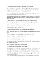
A series of instructions is a program. The
fol-lowing figure shows a basic schematic block
diagram of how a computer works.

Unchanged from the old days, when cards were
read one at a time, computer instructions
con-tinue to be read one at a time. The instruction
is executed, and then the computer goes to the
next instruction. MATLAB executes programs in
this manner as well.

It’s important to realize that the flow of a
program can change. Computers can make

</div>
(26)<div class='page_container' data-page=26>

10

Part I: Getting Started with MATLAB

Using MATLAB as more than a calculator

MATLAB is a computer programming language, not merely a calculator.
However, you can use it like a calculator, and doing so is a good technique to
try ideas that you might use in your program. When you get past the
experi-mentation stage, though, you usually rely on MATLAB to create a program
that helps you perform tasks

✓ Consistently
✓ Easily
✓ Quickly

With these three characteristics in mind, the following sections explore the
idea of MATLAB’s being more than a simple calculator in greater detail. These
sections don’t tell you everything MATLAB can do, but they do provide you
with ideas that you can pursue and use to your own advantage.

Exploring Science, Technology, Engineering, and Mathematics (STEM)

Schools currently have a strong emphasis on Science, Technology, Engineering,
and Math (STEM) topics because the world doesn’t have enough people who
understand these disciplines to get the required work done. Innovation of any
sort requires these disciplines, as do many practical trades. MATLAB has a
rich and large toolbox for STEM that includes

✓ Statistics
✓ Simulation
✓ Image processing
✓ Symbolic processing
✓ Numerical analysis

Performing simple tasks

Many developers start learning their trade using an older language named
Basic. Originally, it was spelled BASIC, for Beginner’s All-Purpose Symbolic
Instruction Code. The intent behind Basic was to make the language simple.
MATLAB retains the simplicity of Basic, but with a much larger toolbox to
solve STEM problems. The idea is that you have better things to do than
learn how to program using a complex language designed to meet needs that
your programs will never address.

</div>
(27)<div class='page_container' data-page=27>

11

Chapter 1: Introducing MATLAB and Its Many Uses

can focus on your work rather than on the tool you’re using to do it. However,
in pursuing simplicity, MATLAB is also less flexible than other programming
languages, provides fewer advanced features for tasks you’ll never perform
anyway, and offers fewer generic tools. MATLAB is designed to meet specific
needs rather than work as a general-purpose language.

Determining why you need MATLAB

It’s important to know how to use any application you adopt, but it’s equally
important to know when to use it and what it can actually do for your
organi-zation. If you don’t have a strong reason to use an application, the purchase
will eventually sit on the shelf collecting dust. This bit of dust collecting
hap-pens far too often in corporations around the world today because people
don’t have a clear idea of why they even need a particular application. Given
that MATLAB can perform so many tasks, you don’t want it to just sit on the
shelf. The following sections can help you build a case for buying and then
using MATLAB in your organization.

Relying on structure for better organization

Writing programs is all about telling the computer to perform a task one step
at a time. The better your language tells the computer what to do, the easier
the computer will be to use and the less time you’ll spend getting it to
per-form a given task.

Starting with the C and Pascal computer languages, developers began
creat-ing structured environments. In such an environment, a map of instructions
and decisions doesn’t look like a bowl of spaghetti — hard to follow and
make sense of — but looks more like a tree, with a trunk and branches that
are much easier to follow and understand. MATLAB places a strong emphasis
on structure (for example, in the way it organizes data and in the manner in
which you write code), which means that you spend a lot more time doing
something fun and a lot less time writing code (because the structure means
that you work with data in a consistent manner).

</div>
(28)<div class='page_container' data-page=28>

12

Part I: Getting Started with MATLAB

Avoiding the complexity of Object-Oriented Programming (OOP)

You may have heard of Object-Oriented Programming (OOP). It’s a discipline
that helps developers create applications based on real-world models. Every
element of an application becomes an object that has specific characteristics
and can perform specific tasks. This technology is quite useful to developers
because it helps them create extremely complex applications with fewer errors
and less coding time.

However, OOP isn’t something you need to know in order to work through
various types of math problems. Even though you can solve difficult math
problems using languages that do support OOP, STEM users can exploit most
of MATLAB’s power without OOP. The lack of an OOP requirement means that
you can get up and running with MATLAB far faster than you could with a
conventional modern programming language and without a loss of the
func-tionality that you need to perform math tasks.

OOP does serve a useful purpose — just not a purpose that you need when
creating math models. Leave the complex OOP languages to developers who
are creating the software used to access huge databases, or developing a new
operating system. MATLAB is designed to make things easy for you.

Using the powerful toolbox

MATLAB provides a toolbox designed to meet the specific needs of STEM
users. In contrast to a general programming language, this toolbox provides
specific functionality needed to meet certain STEM objectives. Here is just
a small sample of the areas that are addressed by the tools you find in the
MATLAB toolbox:

✓ Algebra

✓ Linear algebra — many equations dealing with many unknowns
✓ Calculus

✓ Differential equations
✓ Statistics

✓ Curve fitting
✓ Graphing

✓ Preparing reports

</div>
(29)<div class='page_container' data-page=29>

13

Chapter 1: Introducing MATLAB and Its Many Uses

scene. Nothing is wrong with working directly with the hardware, but you
need specialized knowledge to do it, and writing such code is time
consum-ing. A first-generation language is so hard to use that even the developers
decided to create something better — second-generation languages!
(Second-generation languages, such as Macro Assembler [MASM] are somewhat
human-readable, must be assembled into executable code before use, and are
still specific to a particular processor.)

Most developers today use a combination of third-generation languages such
as C, C++, and Java, and fourth-generation languages such as Structured Query
Language (SQL). A third-generation language gives the developer the kind
of precise control needed to write exceptionally fast applications that can

perform a wide array of tasks. Fourth-generation languages make asking for
information easier. For the MATLAB user, the promise of fourth-generation
languages means being able to work with collections of data, rather than
indi-vidual bits and bytes, making it easier for you to focus on the task, instead of
the language.

As languages progress from first generation to fourth generation (and
beyond), they become more like human language. For example, you might
write something like FIND ALL RECORDS WHERE LAST_NAME EQUALS
‘SMITH’. It’s not quite human language, but close enough that most people
can follow it. You tell the computer what to do, but the computer actually
decides how to do it. Such languages are useful because they take the burden
of interacting with the computer hardware off the language user and place it
on the automation that supports the language.

MATLAB employs a fourth-generation language to make your job a lot
easier. The language isn’t quite human, but it’s also a long way away from
the machine code that developers used to write to make computers work.
Using MATLAB makes you more efficient because the language is specifically
designed to meet the needs of STEM users (just as SQL is designed to meet
the needs of database administrators and developers who need to access
large databases).

Discovering Who Uses MATLAB

for Real-World Tasks

</div>
(30)<div class='page_container' data-page=30>

14

Part I: Getting Started with MATLAB

users whose main goal is productively solving problems in their particular
field — not problems unique to computer programming. You can find MATLAB

used in these kinds of professions:

✓ Scientists
✓ Engineers
✓ Mathematicians
✓ Students
✓ Teachers
✓ Professors
✓ Statisticians
✓ Control technology

✓ Image-processing researchers
✓ Simulation users

Of course, most people want to hear about actual users who are employing
the product to do something useful. You can find such a list at http://www.

mathworks.com/company/user_stories/product.html. Just click the

MATLAB entry to see a list of companies that use MATLAB to perform
real-world tasks. For example, this list tells you that the Centers for Disease Control
(CDC) uses MATLAB for polio virus sequencing (see hworks.

com/company/user_stories/Centers-for-Disease-Control-and-Prevention-Automates-Poliovirus-Sequencing-and-Tracking.
html). You also find that the National Aeronautic and Space Administration
(NASA) used MATLAB when creating the model for the X-43 — the craft that
recently achieved mach 10 (read about it at />

company/user_stories/NASAs-X-43A-Scramjet-Achieves-Record-Breaking-Mach-10-Speed-Using-Model-Based-Design.html). The list

of companies goes on and on. Yes, MATLAB really is used for important tasks by
a large number of companies.

Knowing How to Get the

Most from MATLAB

</div>
(31)<div class='page_container' data-page=31>

15

Chapter 1: Introducing MATLAB and Its Many Uses

money. The following sections provide a brief overview of the skills that are
helpful when working with MATLAB. You don’t need these skills to perform
every task, but they all come in handy for reducing the overall learning curve
and making your MATLAB usage experience nicer.

Getting the basic computer skills

Most complex applications require that you have basic computer skills, such
as knowing how to use your mouse, work with menu systems, understand
what a dialog box is all about, and perform some basic configuration tasks.
MATLAB works like other computer programs you own. It has an intuitive
and conventional Graphical User Interface (GUI) that makes using MATLAB a
lot easier than employing pad and pen. If you’ve learned to use a GUI
operat-ing system such as Windows or the Mac OS X, and you also know how to use
an application such as Word or Excel, you’ll be fine.

This book points out MATLAB peculiarities. In addition, you have access
to procedures that you can use to make your tasks easier to perform. The
combination of these materials will make it easier for you to work with
MATLAB even if your computer skills aren’t as finely honed as they could

be. The important thing to remember is that you can’t break anything when
working with MATLAB. In fact, we encourage trial and error because it’s a
great learning tool. If you find that an example doesn’t quite work as
antici-pated, close MATLAB, reopen it, and start the example over again. MATLAB
and your computer are both more forgiving than others may have led you
to believe.

Defining the math requirements

You need to have the right level of knowledge to use MATLAB. Just as using
SQL is nearly impossible without a knowledge of database management,
using MATLAB is hard without the proper math knowledge. MATLAB’s
ben-efits become evident when applied to trigonometry, exponentials, logarithms,
and higher math.

</div>
(32)<div class='page_container' data-page=32>

16

Part I: Getting Started with MATLAB

Applying what you know about

other procedural languages

One of the more significant problems in understanding how to use any
lan-guage is the procedure. The point was driven home to one fellow at an early
age when his teacher assigned his class the task of writing a procedure for
making toast. Every student carefully developed a procedure for making
toast, and on the day the papers were turned in, the teacher turned up with
a loaf of bread and a toaster. She dutifully followed the instructions each
child provided to the letter. All the children failed at the same point. Yes, they
forgot to take the bread out of the wrapper. You can imagine what it was like
trying to shove a single piece of bread into the toaster when the piece was
still in the wrapper along with the rest of the bread.

Programming can be (at times) just like the experiment with the toast. The
computer takes you at your word and follows to the letter the instructions
you provide. The results may be not what you expected, but the computer
always follows the same logical course. Having previous knowledge of a
pro-cedural language, such as C, Java, C++, or Python, will help you understand
how to write MATLAB procedures as well. You have already developed the
skill required to break instructions into small pieces and know what to do
when a particular piece is missing. Yes, you can use this book without any
prior programming experience, but the prior experience will most definitely
help you get through the chapters must faster and with fewer errors.

Understanding how this book will help you

This is a For Dummies book, so it takes you by the hand to explore MATLAB
and make it as easy to understand as possible. The goal of this book is to help
you use MATLAB to perform at least simple feats of mathematical magic. It
won’t make you a mathematician and it won’t help you become a developer —
those are topics for other books. When you finish this book, you will know
how to use MATLAB to explore STEM-related topics.

Make sure that you also check out the blog for this book at http://blog.

johnmuellerbooks.com/categories/263/matlab-for-dummies.aspx.

</div>
(33)<div class='page_container' data-page=33>

17

Chapter 1: Introducing MATLAB and Its Many Uses

Getting Over the Learning Curve

Even easy programming languages have a learning curve. If nothing else, you
need to discover the techniques that developers use to break tasks into small
pieces, ensure that all the pieces are actually there, and then place the pieces
in a logical order. Creating an orderly flow of steps that the computer can
follow can be difficult, but this book leads you through the process a step at
a time.

</div>
(34)<div class='page_container' data-page=34></div>
(35)<div class='page_container' data-page=35>

Chapter 2

Starting Your Copy of MATLAB

In This Chapter

▶ Obtaining and installing your copy of MATLAB
▶ Starting MATLAB and working with the interface

B

efore you can use MATLAB to do anything productive, you need a copy
of it installed on your system. Fortunately, you can obtain a free trial
version that lasts 30 days. If you’re diligent, you can easily complete this
book in that time and know for certain whether you want to continue using
MATLAB as a productivity aid. The point is that you need a good installation,
and this book helps you obtain that goal.

After you have MATLAB installed, it’s important to introduce yourself to the
interface. This chapter provides you with an overview of the interface, not
a detailed look at every feature. However, overviews are really important
because working with lower-level interface elements is hard if you don’t have
the big picture. You may actually want to mark this chapter in some way so
that you can refer back to the interface information.

Installing MATLAB

A problem that anyone can encounter is getting a bad product installation or
simply not having the right software installed. When you can’t use your
soft-ware properly, the entire application experience is less than it should be. The
following sections guide you through the MATLAB installation so that you can
have a great experience using it.

Discovering which platforms

MATLAB supports

</div>
(36)<div class='page_container' data-page=36>

20

Part I: Getting Started with MATLAB

resources, but you won’t be happy with the performance.) You also need to
know which platforms MATLAB supports. You can use it on these systems:

✓ Windows (3GB free disk space, 2GB RAM)
• Windows 8.1

• Windows 8

• Windows 7 Service Pack 1
• Windows Vista Service Pack 2
• Windows XP Service Pack 3

• Windows XP x64 Edition Service Pack 2
• Windows Server 2012

• Windows Server 2008 R2 Service Pack 1

• Windows Server 2008 Service Pack 2
• Windows Server 2003 R2 Service Pack 2
✓ Mac OS X

• Mac OS X 10.9 (Mavericks)
• Mac OS X 10.8 (Mountain Lion)
• Mac OS X 10.7.4+ (Lion)
✓ Linux

• Ubuntu 12.04 LTS, 13.04, and 13.10
• Red Hat Enterprise Linux 6.x

• SUSE Linux Enterprise Desktop 11 SP3
• Debian 6.x

Linux users may find that other distributions work. However, the list of Linux
systems represents those that are tested to work with MATLAB. If you try
MATLAB on your unlisted Linux system and find that it works well, please
let John know (at ) and he’ll mention these
other systems in a blog post. The point is that you really do need to have the
right platform to get good results with MATLAB. You can always obtain the
current minimum requirements for MATLAB at hworks.

com/support/sysreq/current_release/index.html.

Getting your copy of MATLAB

</div>
(37)<div class='page_container' data-page=37>

21

Chapter 2: Starting Your Copy of MATLAB

✓ Get the trial version from />

trials/trial_request.html.

✓ Obtain a student version of the product from hworks.

com/academia/student_version/.

✓ Buy a copy from />index.html.

In most cases, you need to download the copy of MATLAB or the MATLAB
installer onto your system after you fill out the required information to get it.
Some users choose to receive a DVD in the mail instead of downloading the
product online. No matter which technique you use, you eventually get a copy
of MATLAB to install.

Performing the installation

The method you use to install MATLAB depends on the version you obtain
and the media used to send it to you. For example, there is a method for
installing MATLAB from DVD and an entirely different method when you want
to download the installer and use an Internet connection. Administrators and
users also have different installation procedures. Use the table at http://

www.mathworks.com/help/install/ug/choose-installation-procedure.html to determine which installation procedure to use.
MathWorks provides you with substantial help in performing the
installa-tion. Before you contact anyone, be sure to look through the materials on the
main installation page at />index.html. It’s also possible to obtain installation help at http://www.

mathworks.com/support/install-matlab.html. Take the time to review

the material that MathWorks provides before you push the panic button. Doing
so will save time and effort.

Activating the product

After you complete the MATLAB installation, you must activate the product.
Activation is a verification process. It simply means that MathWorks verifies
that you have a valid copy of MATLAB on your system. With a valid copy, you
obtain support such as updates to your copy of MATLAB as needed.

As with installation, you have a number of activation types to use with MATLAB
that depend on the product version and how you’re using the product. The chart

</div>
(38)<div class='page_container' data-page=38>

22

Part I: Getting Started with MATLAB

license-option-and-activation-type-matrix.html tells you whether

your particular version of MATLAB supports a specific activation type. For
example, the individual license doesn’t support the Network Named User
activation type.

MATLAB automatically asks you about activation after the installation process
is complete. You don’t need to do anything special. However, you do want to
consider the type of activation you want to perform — which type of
activa-tion will best meet your needs and those of your organizaactiva-tion.

Meeting the MATLAB Interface

Most applications have similar interface functionality. For example, if you
click a button, you expect something to happen. The button usually contains
text that tells you what will happen when you click it, such as closing a dialog
box by clicking OK or Cancel. However, the similarities aren’t usually enough
to tell you everything you need to know about the interface. The following
sections provide an overview of the MATLAB interface so that you can work
through the chapters that follow with greater ease. These sections don’t tell
you everything about the interface, but you do get enough information to feel
comfortable using MATLAB.

Starting MATLAB for the first time

When you start MATLAB for the first time (after you activate it), you see a
display containing a series of blank windows. It’s not all that interesting just
yet because you haven’t done anything with MATLAB. However, each of the
windows has a special purpose, so it’s important to know which window to
use when you want to perform a task.

It’s possible to arrange the windows in any order needed. Figure 2-1 shows
the window arrangement used throughout the book, which may not precisely
match your display. The “Changing the MATLAB layout” section of this chapter
tells you how to rearrange the windows so that you can see them the way that
works best when you work. Here is a brief summary of the window functionality.

</div>
(39)<div class='page_container' data-page=39>

23

Chapter 2: Starting Your Copy of MATLAB

Figure 2-1:

The initial
view of
MATLAB
is pretty
much empty
space.

✓ Quick Access toolbar: The Quick Access toolbar (QAT) provides access
to the MATLAB features that you use most often. Finding icons on the
QAT is often faster and easier than looking them up on the Toolstrip.
You can change the QAT to meet your needs. To add an icon to the QAT,

right-click its entry in the Toolstrip and choose Add to Quick Access
Toolbar from the context menu. If you want to remove an icon from the
QAT, right-click its entry in the QAT and choose Remove from the Quick
Access Toolbar from the context menu.

✓ Minimize Toolstrip: If you find that the Toolstrip is taking up too much
space, you can click the Minimize Toolstrip icon to remove it from view.
To restore the Toolstrip, simply click the Minimize Toolstrip icon again.
When the Toolstrip is minimized, you can still see the three tabs —

</div>
(40)<div class='page_container' data-page=40>

24

Part I: Getting Started with MATLAB

✓ Command window: You type formulas and commands in this window.
After you type the formula or command and press Enter, MATLAB
deter-mines what it should do with the information you typed. You see the
Command window used later in this chapter.

✓ Workspace window: The Workspace window contains the results of any

tasks you ask MATLAB to perform. It provides a scratchpad of sorts that
you use for calculations. The Workspace window and Command window
work hand in hand to provide you with a complete view of the work you
perform using MATLAB.

✓ Command History window: In some cases, you want to reissue a
for-mula or command. The Command History window acts as your memory
and helps you restore formulas and commands that you used in the
past. You see the Command History window used later in this chapter.
✓ Status bar: It’s important to know the current MATLAB state — whether

MATLAB is ready to perform additional work or not. The status bar
nor-mally contains one word, Ready, which tells you that MATLAB is ready
to perform tasks. However, you need to watch this window when
per-forming complex tasks to see what MATLAB is doing at any given time.
✓ Details window: The Details window shows specifics about any file you

select in the Current Folder window.

✓ Current Folder window and Address Field: The Current Folder window
contains a listing of the files you’ve created in the current folder — files
you’d use to store any data you create in MATLAB, along with any scripts
or functions you’d use to manipulate data). The Current Folder is listed
in the Address Field text box that appears directly below the Toolstrip.
Changing the Address Field text box content also changes the content of
the Current Folder window.

Employing the Command window

The Command window is where you perform most of your experimentation.

This chapter shows how to perform really simple tasks using the Command
window, but as the book progresses, you see that the Command window can
do quite a lot for you. The following sections describe some of the ways in
which you can use the Command window to learn more about MATLAB.

Typing a really simple command

You can type any formula or command desired in the Command window and
see a result. Of course, it pays to start with something really simple so that
you can get the feel of how this window works. Type 2 + 2 and press Enter in
the Command window. You see the results shown in Figure 2-2.

</div>
(41)<div class='page_container' data-page=41>

25

Chapter 2: Starting Your Copy of MATLAB

Figure 2-2: 
A very
simple

com-mand in
MATLAB.

✓ Command window: Receives the output of the formula 2 + 2, which
is ans = 4. MATLAB assigns the output of the formula to a variable
named ans. Variables are boxes (pieces of memory) in which you can
place data. In this case, the box contains the number 4.

✓ Workspace window: Contains any variables generated as the result of
working in the Command window. In this case, the Workspace window
contains a variable named ans that holds a value of 4.

Notice that the variable can’t contain any other value than 4 because the Min
column also contains 4, as does the Max column. When a variable can
con-tain a range of values, the minimum value that it can concon-tain appears in the
Min column and the maximum value that it can contain appears in the Max
column. The Value column always holds the current value of the variable.
✓ Command History window: Displays the series of formulas or

com-mands that you type, along with the date and time you typed them. You
can replay a formula or command in this window. Just select the formula
or command that you want to use from the list to replay it.

Getting additional help

</div>
(42)<div class='page_container' data-page=42>

26

Part I: Getting Started with MATLAB

✓ Watch This Video: Opens a tutorial in your browser. The video provides
a brief introduction to MATLAB. Simply watch it for a visual presentation
of how to work with MATLAB.

✓ See Examples: Displays a Help dialog box that contains an assortment of
examples that you can try, as shown in Figure 2-3. The examples take a
number of forms:

• Video: Displays a guided presentation of how to perform a task that
opens in your browser. The length of time of each video is listed
next to its title.

• Script: Opens the Help dialog box to a new location that contains
an example script that demonstrates some MATLAB feature and an

explanation of how the script works. You can open the script and
try it yourself. Making changes to the script is often helpful to see
how the change affects script operation.

• App: Starts a fully functional app that you can use to see how
MATLAB works and what you can expect to do with it.

Figure 2-3: 
The

exam-ples give
you
practi-cal
experi-ence using

</div>
(43)<div class='page_container' data-page=43>

27

Chapter 2: Starting Your Copy of MATLAB

✓ Read Getting Started: Displays a Help dialog box that contains
addi-tional information about MATLAB, such as the system requirements, as
shown in Figure 2-4. You also gain access to a number of tutorials.

Figure 2-4: 
The Getting
Started

informa-tion helps
you learn
more about

MATLAB
and
pro-vides
access to
tutorials.

Using the Current Folder toolbar

The Current Folder toolbar helps you navigate the Current Folder window
with greater precision. Here is a description of each of the toolbar elements
when viewed from left to right on the toolbar:

✓ Back: Moves you back one entry in the file history listing. MATLAB
retains a history of the places you visit on the hard drive. You can move
backward and forward through this list to get from one location to
another quite quickly.

✓ Forward: Moves you forward one entry in the file history listing.
✓ Up One Level: Moves you one level up in the directory hierarchy. For

</div>
(44)<div class='page_container' data-page=44>

28

Part I: Getting Started with MATLAB

✓ Browse for Folder: Displays a Select a New Folder dialog box that you
can use to view the hard drive content. Highlight the folder you want to
use and click Select to change the Current Folder window location to the
selected folder.

✓ Address field: Contains the current folder information. Type a new value
and press Enter to change the folder.

✓ Search (the Magnifying Glass icon to the right of the Address field):

Changes the Address field into a search field. Type the search criteria
that you want to use, press Return, and MATLAB displays the results for
you in the Current Folder window.

Viewing the Current Folder window

The Current Folder window (refer to Figure 2-1) really does show the current
folder listed in the Address field. You don’t see anything because the current
folder has no files or folders to display. However, you can add files and
fold-ers as needed to store your MATLAB data.

When you first start MATLAB, the current folder always defaults to the MATLAB
folder found in your user folder for the platform of your choice. For Windows
users, that means the C:\Users\<User Name>\Documents\MATLAB folder
(where <User Name> is your name). Burying your data way down deep in the
operating system may seem like a good idea to the operating system vendor,
but you can change the current folder location to something more convenient
when desired. The following sections describe techniques for managing data
and its storage location using MATLAB.

Temporarily changing the current folder

There are times when you need to change the current folder. Perhaps your
data is actually stored on a network drive, you want to use a shared location
so that others can see your data, or you simply want to use a more
conven-ient location on your local drive. The following steps help you change the
current folder:

1. Click Set Path in the Environment group on the Toolstrip’s Home tab.

You see the Set Path dialog box shown in Figure 2-5.

This dialog box lists all the places the MATLAB searches for data, with
the default location listed first. You can use these techniques to work
with existing folders (go to Step 3 when you’re finished):

• To set an existing folder as the default folder, highlight the folder in
the list and click Move to Top.

</div>
(45)<div class='page_container' data-page=45>

29

Chapter 2: Starting Your Copy of MATLAB

2. Click Add Folder.

You see the Add Folder to Path dialog box, as shown in Figure 2-6.
Figure 2-5:

The Set Path
dialog box
contains
a listing of
folders that
MATLAB
searches for
data.

</div>
(46)<div class='page_container' data-page=46>

30

Part I: Getting Started with MATLAB

This dialog box lets you choose an existing folder that doesn’t appear in
the current list or add a new folder to use:

• To use a folder that exists on your hard drive, use the dialog box’s
tree structure to navigate to the folder, highlight its entry, and then
click Select Folder.

• To create a new folder, highlight the parent folder in the dialog
box’s tree structure, click New Folder, type the name of the folder,
press Enter, and then click Select Folder.

3. Click Save.

MATLAB makes the folder you select the new default folder. (You may
see a User Account Control dialog box when working with Windows;
click Yes to allow Windows to perform the task.)

4. Click Close.

The Set Path dialog box closes.

5. Type the new location in the Address field.

The Current Folder display changes to show the new location.

Permanently changing the default folder

The default folder is the one that MATLAB uses when it starts. Setting a default
folder saves you time because you don’t have to remember to change the
current folder setting every time you want to work. If you have your default

folder set to the location from which you work most of the time, you can usually
get right to work and not worry too much about locations on the hard drive.
If you want to permanently change the default folder so that you see the
same folder every time you start MATLAB, you must use the userpath()
command. Even though this might seem like a really advanced technique,
it isn’t hard. In fact, go ahead and set the userpath so that it points to the
downloadable source for this book. Simply type userpath(‘C:\MATLAB’) in
the Command window and press Enter. You need to change the path to
wher-ever you placed the downloadable source.

To see what the default path is for yourself, type userpath and press Enter.
MATLAB displays the current default folder.

Creating a new folder

</div>
(47)<div class='page_container' data-page=47>

31

Chapter 2: Starting Your Copy of MATLAB

Each chapter in this book uses a separate folder to store any files you create.
When you obtain the downloadable source from the publisher’s site (http://
www.dummies.com/extras/matlab), you find the files for this chapter in
the \MATLAB\Chapter02 folder. Every other chapter will follow the same
pattern.

Saving a formula or command as a script

After you create a formula or command that you want to use to perform a
number of calculations, be sure to save it to disk. Of course, you can save
anything that you want to disk, even the simple formula you typed earlier in

this chapter. The following steps help you save any formula or command that
you want to disk so that you can review it later:

1. Choose a location to save the formula or command in the Address 
field.

2. Right-click the formula or command that you want to save in the 
Command History window and choose Create Script from the context 
menu.

You see the Editor window, as shown in Figure 2-7. The script is
cur-rently untitled, so you see the script name as Untitled*. (Figure 2-7
shows the Editor window undocked so you can see it with greater
ease — the “Changing the MATLAB layout” section of this chapter tells
how to undock windows so you can get precisely the same look.)

Figure 2-7: 
The Editor
turns your
formula or
command
into a script.

</div>
(48)<div class='page_container' data-page=48>

32

Part I: Getting Started with MATLAB

3. Click Save on the Editor tab.

You see the Select File for Save As dialog box, as shown in Figure 2-8.

Figure 2-8:

Choose a
location to
save your
script and
provide a
filename
for it.

4. In the left pane, highlight the location you want to use to save 
the file.

5. Type a name for the script in the File Name field.

The example uses FirstScript.m. However, when you save your own
scripts, you should use a name that will help you remember the content
of the file. Descriptive names are easy to remember and make precisely
locating the script you want much easier later.

MATLAB filenames can contain only letters and numbers. You can’t use
spaces in a MATLAB filename. However, you can use the underscore in
place of a space.

6. Click Save.

MATLAB saves the script for you so that you can reuse it later. The title
bar changes to show the script name and its location on disk.

7. Close the Editor window.

</div>
(49)<div class='page_container' data-page=49>

33

Chapter 2: Starting Your Copy of MATLAB

Figure 2-9: 
The Current
Folder
window
always
shows the
results of
any changes
you make.

Running a saved script

You can run any script by right-clicking its entry in the Current Folder window
and choosing Run from the context menu. When you run a script, you see the
script name in the Command window, the output in the Workspace window,
and the actual command in the Command History window, as shown in
Figure 2-10.

Saving the current workspace to disk

Sometimes you might want to save your workspace to protect work in
prog-ress. The work may not be ready to turn into a script, but you want to save it
before quitting for the day or simply to ensure that any useful work isn’t
cor-rupted by errors you make later.

To save your workspace, click Save Workspace in the Variable group of the
Toolstrip’s Home tab. You see a Save to MAT-file dialog box that looks similar

to the Select File for Save As dialog box (refer to Figure 2-8). Type a filename
for your workspace, such as FirstWorkspace.mat, and click Save to save it.
Workspaces use a .mat extension, while scripts have a .m extension. Make
sure that you don’t confuse the two extensions. In addition, workspaces and
scripts use different icons so that you can easily tell them apart in the Current
Folder window.

Changing the MATLAB layout

</div>
(50)<div class='page_container' data-page=50>

34

Part I: Getting Started with MATLAB

Figure 2-10: 
Running a
script shows
its name and
results.

Minimizing and maximizing windows

Sometimes you need to see more or less of a particular window. It’s possible
to simply resize the windows, but you may want to see more or less of the
window than resizing provides. In this case, you can minimize the window to
keep it open but completely hidden from view, or maximize the window to
allow it to take up the entire client area of the application.

On the right side of the title bar for each window, you see a down arrow. When
you click this arrow, you see a menu of options for that window, such as the
options shown in Figure 2-11 for the Current Folder window. To minimize a
window, choose the Minimize option from this menu. Likewise, to maximize a
window, choose the Maximize option from the menu.

Eventually, you want to change the window size back to its original form.
The Minimize or Maximize option on the menu is replaced by a Restore
option when you change the window’s setup. Select this option to restore the
window to its original size.

Opening and closing windows

</div>
(51)<div class='page_container' data-page=51>

35

Chapter 2: Starting Your Copy of MATLAB

accessible. To close a window that you don’t need, click the down arrow on
the right side of the window and choose Close from the menu.

Figure 2-11: 
The window
menus
con-tain options
for changing
the

appear-ance of the
window.

After you close a window, the down arrow is no longer accessible, so you can’t
restore a closed window by using the menu options shown in Figure 2-11.
To reopen a window, you click the down arrow on the Layout button in the
Environment group of the Home tab. You see a list of layout options like the
ones shown in Figure 2-12.

The Show group contains a listing of windows. Each window with a check
mark next to it is opened for use (closed windows have no check mark). To
open a window, click its entry. Clicking the entry places a check next to that
window and opens it for you. The window is automatically sized to the size it
was the last time you had it open.

You can also close windows using the options on the Layout menu. Simply
click the check next to a window entry to close it.

Docking and undocking windows

Many people have multiple monitors attached to their systems. It’s often
more efficient to perform the main part of your work on your main monitor
and move supplementary windows to a second monitor. However, you really
can’t move a window until you undock the window from MATLAB so that you
can move just that window to another location.

</div>
(52)<div class='page_container' data-page=52>

36

Part I: Getting Started with MATLAB

Figure 2-12: 
The Layout
menu
contains
the layout
options for
MATLAB.

At some point, you may decide that you want MATLAB to have all its
win-dows in one place again. In this case, you click the down arrow on the right

side of the window’s title bar and choose Dock from the menu. MATLAB
places the window precisely where it was before you undocked it. However,
the window may not return to its original size — you may need to resize it to
make it fit as it did before.

Choosing an existing layout

One of the potential problems of changing your layout is that it may cause
MATLAB to become nearly unusable. Rather than spend a lot of time trying to
get the original layout back, you can simply choose an existing layout. To
per-form this task, click the down arrow on the Layout button in the Environment
group of the Home tab and choose one of the Select Layout options. The
Default entry returns MATLAB to the same state it was in when you started it
the first time.

Saving a new layout

</div>
(53)<div class='page_container' data-page=53>

Chapter 3

Interacting with MATLAB

In This Chapter

▶ Performing basic calculations
▶ Creating more complex calculations
▶ Interacting with variables

▶ Using MATLAB functions
▶ Overcoming errors
▶ Obtaining additional help

Y

ou can interact with MATLAB in a lot of ways and you’ll experience
quite a few of them as the book progresses. However, it pays to start out
slowly to build your skills. This chapter presents an overview of the sorts of
things you can do with MATLAB. Use this chapter to get started with a
prod-uct that can really perform complex tasks with aplomb.

</div>
(54)<div class='page_container' data-page=54>

38

Part I: Getting Started with MATLAB

In the process of interacting with MATLAB, you’ll make mistakes. Of course,
everyone makes mistakes. MATLAB won’t blow up if you make a mistake, and
your computer won’t up and run away. Mistakes are part of the learning process,
so you need to embrace them. In fact, most of the greatest people in history
made a ton of mistakes (see Defining the Benefits of Failure at http://blog.

johnmuellerbooks.com/2013/04/26/defining-the-benefits-of-failure/). This book assumes that you’re going to make mistakes, so part
of this chapter discusses how to recover from them. Knowing how to recover
means that you don’t have to worry about making a mistake because you can
always start fresh.

And finally in this chapter is the topic of additional resources for finding
help. No one wants to reinvent the wheel, and a lack of progress can become
discouraging after a while. That’s why you’ll definitely want to know where to
find help on using MATLAB. The final section of this chapter discusses
tech-niques you can use to obtain additional help. Working through issues with
MATLAB on your own is important because that’s how you learn. However,
after you’ve worked through the issues for a while, you also need to know
where to get additional help.

Using MATLAB as a Calculator

MATLAB performs math tasks incredibly well. Sometimes people get so
caught up in “what else” an application can do that they miss the most
interesting facts that are staring them right in the face. The following
sec-tions help you understand MATLAB as a calculator so that you can use it
for experimentation purposes.

Entering information at the prompt

References to using the prompt appear a few times in previous chapters, but
those chapters don’t fully explain it. The prompt is that place where you type
formulas, commands, or functions or perform tasks using MATLAB. It appears
in the Command window. Normally, the prompt appears as two greater-than
signs (>>). However, when working with some versions of MATLAB, you might
see EDU>> (for the student version) or Trial>> (for the trial version) instead.
No matter what you see as a prompt, you use it to know where to type the
information described in this book.

</div>
(55)<div class='page_container' data-page=55>

39

Chapter 3: Interacting with MATLAB

Type clc and press Enter at the MATLAB prompt. If the Command window
con-tains any information, MATLAB clears it for you.

The userpath() function is called a function because it uses parentheses
to hold the data — also called arguments — you send to MATLAB. The clc
command is a command because you don’t use parentheses with it. Whether
something is a function or a command depends on how you use it. The usage
is called the function or command syntax (the grammar used to tell MATLAB

what tasks to perform). It’s possible to use userpath() in either Function
or Command form. To avoid confusion, the book usually relies on function
syntax when you need to provide arguments, and command syntax when you
don’t. So, when you see parentheses, you should also expect to provide input
with the function call (the act of typing the function and associated
argu-ments, and then pressing Enter).

MATLAB is also case sensitive. That sounds dangerous, but all it really means
is that CLC is different from Clc, which is also different from clc. Type CLC

and press Enter at the MATLAB prompt. You see an error message like the one
shown in Figure 3-1. (MATLAB will also suggest the correct command, clc, but
ignore the advice for right now by highlighting clc and pressing Delete.) Next,
type Clc and press Enter at the MATLAB prompt. This time, you see the same
error because you made the “same” mistake — at least in the eyes of MATLAB.
If you see this error message, don’t become confused simply because MATLAB
didn’t provide a clear response to what you typed — just retype the command,
being sure to type the command exactly as written.

Figure 3-1: 
MATLAB is
case
sensi-tive, so CLC,

Clc, and clc
all mean
different
things.

</div>
(56)<div class='page_container' data-page=56>

40

Part I: Getting Started with MATLAB

prompt to determine whether help is available.) Because MATLAB was able
to provide the correct command in this case, simply press Enter to clear the
Command window.

Look in the Command History window. Notice that there is a red line next to
each of the errant commands you typed. These red lines tell you when you
shouldn’t use a command or function again because it produced an error the
first time. You should also avoid adding errant commands and functions to
any scripts you create.

Entering a formula

To enter a formula, you simply type it. For example, if you type 2 + 2 and press
Enter, you get an answer of 4. Likewise, if you type 2 * pi * 6378.1 and press
Enter, you get the circumference of the earth in km (see c.
nasa.gov/planetary/factsheet/earthfact.html for a list of Earth
sta-tistics, including radius). The second formula uses a predefined constant, pi,
which equals 3.1416. MATLAB actually defines a number of predefined constants
that you can use when entering a formula:

✓ ans: Contains the most recent temporary answer. MATLAB creates this
special temporary variable for you when you don’t provide a variable of
your own.

✓ eps: Specifies the accuracy of the floating-point precision (epsilon),
which defaults to 2.2204e-16.

✓ i: Contains an imaginary number, which defaults to 0.0000 + 1.0000i.
✓ Inf: Defines a value of infinity, which is any number divided by 0, such

as 1 / 0.

✓ NaN: Specifies that the numerical result isn’t defined (Not a Number).
✓ pi: Contains the value of pi, which is 3.1416 when you view it onscreen.

Internally, MATLAB stores the value to 15 decimal places so that you’re
assured of accuracy.

</div>
(57)<div class='page_container' data-page=57>

41

Chapter 3: Interacting with MATLAB

Copying and pasting formulas

With MATLAB, you can copy and paste formulas that you create into other
documents (such as a script or function file, or to another application). To
begin, you highlight the information you want to copy. Use one of these
meth-ods to copy the text after you highlight it:

Figure 3-2: 
Any formula
you enter
changes
the content
of ans.

✓ Click Copy on the QAT.

✓ Right-click the highlighted text and choose Copy from the context menu.

✓ Rely on a platform-specific method of copying the text, such as pressing

Ctrl+C on Windows.

When you have the text on the Clipboard, you can paste it wherever you want.
If you want to paste it somewhere in MATLAB, click wherever you want to put
the text, such as after the prompt. Use one of these methods to paste the text:

✓ Click Paste on the QAT.

✓ Right click the insertion point and choose Paste from the context menu.
✓ Rely on a platform-specific method of pasting text, such as pressing

</div>
(58)<div class='page_container' data-page=58>

42

Part I: Getting Started with MATLAB

Changing the Command window formatting

The Command window provides the means necessary to change the output
formatting. For example, if you don’t want the extra space between lines that
MATLAB provides by default, you can type format compact and press Enter
to get rid of it. In fact, try typing that command now. When you type format

Understanding integer and floating-point values

Throughout the book, you see the terms integer

and floating point. These two terms describe
kinds of numbers. When most people look at 3
and 3.0, they see the same number: the value
three. The computer, however, sees two

dif-ferent numbers. The first is an integer — a
number without a decimal portion. The second
is a floating-point value — a number that has
a decimal portion, even if it’s a whole number.
You see these two terms often in this book
because the computer works with and stores
integer values differently from floating-point
values. How the computer interacts differently
with them is not important — you just need to
know that it does. MATLAB does a great job of
hiding the differences from view unless the
dif-ference becomes important for some reason,
such as when you want to perform integer
math — in which you want to work with only
whole numbers. For example, 4 divided by 3 is
equal to 1 with a remainder of 1 when
perform-ing integer math.

Humans also don’t pay much attention to the
size of a number. Again, the computer must do
so because it has to allocate memory to hold
the number — and larger numbers require
more memory. So, not only do you need to
con-sider the kind of number but also the size of the
number when performing some tasks.

Finally, the computer must also consider
whether a number has a sign associated with
it. The sign takes up part of the memory used

to store the number. If you don’t need to store
a sign, the computer can use that memory to
store additional number information. With all
these points in mind, here are the kinds of
num-bers that MATLAB understands:

✓ double: 64-bit floating-point double precision
✓ single: 32-bit floating-point double precision

✓ int8: 8-bit signed integer
✓ int16: 16-bit signed integer
✓ int32: 32-bit signed integer
✓ int64: 64-bit signed integer

✓ uint8: 8-bit signed integer
✓ uint16: 16-bit signed integer
✓ uint32: 32-bit signed integer
✓ uint64: 64-bit signed integer

</div>
(59)<div class='page_container' data-page=59>

43

Chapter 3: Interacting with MATLAB

compact and press Enter, you don’t see any output. However, the next
for-mula you type shows the difference. Type 2 + 2 and press Enter. You see that
the extra spaces between lines are gone, as shown in Figure 3-3.

Figure 3-3: 
Modify the

appear-ance of the

Command
window
using format
commands.

MATLAB provides a number of format commands. Each of them begins with
the keyword format, followed by an additional instruction. Here is a list of
the instructions you can type:

✓ short: All floating-point output has at least one whole number, a decimal
point, and four decimal values, such as 4.2000.

✓ long: All floating-point output has at least one whole number, a decimal
point, and 15 decimal values, such as 4.200000000000000.

✓ shorte: All floating-point output uses exponential format with four
decimal places, such as 4.2000e+00.

✓ longe: All floating-point output uses exponential format with 15 decimal
places, such as 4.200000000000000e+00.

✓ shortg: All output uses a short general format, such as 4.2, with five
digits of space.

✓ long: All output uses a long general format, such as 4.2, with 15 digits of
space.

✓ shorteng: All floating-point output uses exponential format with four

decimal places and powers in groups of three, such as 4.2000e+000.
✓ longeng: All floating-point output uses exponential format with 14 decimal

places and powers in groups of three, such as 4.20000000000000e+000.
✓ hex: All output is in hexadecimal format, such as 4010cccccccccccd.
✓ +: All output is evaluated for positive or negative values, so that the

result contains just a + or - sign, such as + when using the formula 2 * 2.1.
✓ bank: All output provides two decimal places, even for integer

</div>
(60)<div class='page_container' data-page=60>

44

Part I: Getting Started with MATLAB

✓ rat: All output is presented as a ratio of small integers, such as 21/5
for 4.2.

✓ compact: All output appears in single-spaced format.
✓ loose: All output appears in double-spaced format.

Suppressing Command window output

When performing most experiments, you want to see the result of your
actions. However, sometimes you really don’t want to keep seeing the results
in the Command window when you can just as easily look in the Workspace
window for the result. In these cases, you can follow a command with a
semi-colon (;) and the Command window output is suppressed. For example, try
typing 2 + 2; and pressing Enter (note the semicolon at the end of the
com-mand). You see output similar to that in Figure 3-4.

Figure 3-4: 
Use a

semicolon
to hide the
results of an
action in the
Command
window.

Now look at the Workspace window. The results are shown there just as you
would expect. This technique is often used when you have a complex set of
formulas to type and you don’t want to see the intermediate results or when
working with large matrices. Of course, you also want to use this approach
when you create scripts so that the script user isn’t bombarded by the
results that will appear as the script runs. Anytime you stop using the
semi-colon at the end of the command, you start seeing the results again.

</div>
(61)<div class='page_container' data-page=61>

45

Chapter 3: Interacting with MATLAB

MATLAB rules as well. The following sections get you started with the basics
that you use to build an understanding of the MATLAB language. You may be
surprised to find that you already know some of these rules, and other rules
are simply extensions of those rules.

Adding, subtracting, multiplying,

and dividing

MATLAB is a math-based language, so it pays to review the basic rules for
telling MATLAB how to perform basic math tasks. Of course, MATLAB
per-forms the basic math functions:

✓ + or plus(): Adds two numbers. For example, you can use 3 + 4 or
plus(3, 4) to obtain a result of 7.

✓ - or minus(): Subtracts two numbers. For example, you can use 3 - 4
or minus(3, 4) to obtain a result of –1.

✓ * or times(): Multiplies two numbers. For example, you can use 3 * 4
or times(3, 4) to obtain a result of 12.

✓ / or rdivide(): Performs right division, which is the form of division
you likely learned in school. For example, you can use 3 / 4 or
rdivide(3, 4) to obtain a result of 0.75.

✓ \ or ldivide(): Performs left division, which is also called “goes into”
or, as you learned in third grade, “guzintas.” You know (say this out loud),
5 “guzinta” 5 once, 5 “guzinta” 10 twice, 5 “guzinta” 15 three times, and
so on. For example, you can use 3 \ 4 or ldivide(3, 4) to obtain a
result of 1.3333.

Most MATLAB operators are binary, which means that they work on two
values. For example, 3 + 4 has two values: 3 and 4. However, some
opera-tors are unary, which means that they work on just one value. Here are the
basic unary operators:

✓ + or uplus(): Returns the unmodified content of a value or variable.
For example, +1 or uplus(1) is still equal to 1.

✓ - or uminus(): Returns the negated content of a value or variable. For
example, -1 or uminus(1) returns –1. However, -–1 or uminus(–1)

returns 1 (the negative of a negative is a positive).

</div>
(62)<div class='page_container' data-page=62>

46

Part I: Getting Started with MATLAB

✓ idivide(): Performs integer division. You supply two values or
vari-ables as input, along with an optional modifier that tells MATLAB how to
perform rounding.

To use the idivide() function, you must specify that the input values
are integers (see the “Understanding integer and floating-point values”
sidebar in this chapter for details). For example, idivide(int32(5),
int32(3)) provides an output of 1. Here is a list of the modifiers you
use to provide different rounding effects:

• ceil: Rounds toward positive infinity. For example, idivide

(int32(5), int32(3), 'ceil') produces an output of 2

and idivide(int32(5), int32(–3), 'ceil') produces an

output of –1.

• fix: Rounds toward zero. For example, idivide(int32(5),
int32(3), 'fix') produces an output of 1 and idivide
(int32(5), int32(–3), 'fix') produces an output of –1.

• floor: Rounds toward negative infinity. For example, idivide

(int32(5), int32(3), 'floor') produces an output of 1 and

idivide(int32(5), int32(–3), 'floor') produces a result

of –2.

• round: Rounds to the nearest integer. For example, idivide

(int32(5), int32(3), 'round') produces an output of 2

and idivide(int32(5), int32(–3), 'round') produces an

output of –2.

✓ mod(): Obtains the modulus after division. For example, mod(5, 3)
produces an output of 2 and mod(5, –3) produces an output of –1.
✓ rem(): Obtains the remainder after division. For example, rem(5, 3)

produces an output of 2 and rem(5, –3) produces an output of –2.
Rounding can be an important feature of an application because it
deter-mines the approximate values the user sees. You can round any formula that
you want to produce an integer output. Here are the rounding functions:

✓ ceil(): Rounds toward positive infinity. For example, ceil(5 / 3)
produces an output of 2 and ceil(5 / –3) produces an output of –1.
✓ fix(): Rounds toward zero. For example, fix(5 / 3) produces an

output of 1 and fix(5 / –3) produces an output of –1.

✓ floor(): Rounds toward negative infinity. For example, floor(5 / 3)
produces an output of 1 and floor(5 / –3) produces an output of –2.
✓ round(): Rounds toward nearest integer. For example, round(5 / 3)

</div>
(63)<div class='page_container' data-page=63>

47

Chapter 3: Interacting with MATLAB

Working with exponents

You use the caret (^) to raise a number to a particular power. MATLAB can
handle negative, fractional, and complex number bases as exponents. Here
are some examples of exponents:

✓ 10^3 = 1000
✓ 2^10 = 1024
✓ 2.5^2.5 = 9.8821
✓ 2^-4 = 0.0625

✓ 2^I = 0.7692 + 0.6390i
✓ i^I = 0.2079

Why we use the letter

E

(or

e

) for scientific

notation

In the early days of computing, a display would
use seven Light Emitting Diode (LED), or Liquid
Crystal Display (LCD) segments to display
num-bers by turning particular segments on or off.
Even today, many watches and clocks use this
technique. The following figure shows how a
seven-segment display works.

When designers made calculators that
dis-played scientific notation, they thought of the
letter E, which reminds users that what follows
is an exponent. They could also implement E

using a seven- segment display, as shown here:

Then designers got lazy and instead
of letting uppercase E mean
scien-tific notation, they also let a
lower-case e mean the same thing. In our
modern age, designers can use all

the pixels that various screens now employ to
display the information without using the letter

</div>
(64)<div class='page_container' data-page=64>

48

Part I: Getting Started with MATLAB

Organizing Your Storage Locker

Computers contain memory, much as your own brain contains memory. The
computer’s memory stores information that you create using MATLAB. Looking
at memory as a kind of storage locker can be helpful. You open the door, put
something inside and then close the door until you need the item again. When
that happens, you simply open the door and take the item out. The idea of
memory doesn’t have to be complex or difficult to understand.

Whenever you tell MATLAB to store something in memory, you’re using a
variable. Developers use the term variable to indicate that the content of the
memory isn’t stable — it can change. The following sections tell you more

about the MATLAB storage lockers called variables.

Using ans — the default storage locker

MATLAB always needs a place to store the output of any calculation you
perform. For example, when you type 2 + 2 and press Enter, the output tells
you that the value is 4. However, it more specifically tells you that ans = 4.
MATLAB uses ans as a storage locker when you don’t specify a specific
stor-age locker to use.

MATLAB uses ans as a temporary storage locker. The content lasts only as
long as you keep MATLAB open and you don’t perform another calculation
that requires ans to hold the output. If you need the result from a calculation
for additional tasks, you must store the result in another variable.

Creating your own storage lockers

Whenever you need to use the result of a calculation in future calculations,
you must create your own storage locker to hold the information; using the
ans temporary variable just won’t work. Fortunately, creating your own
vari-ables is straightforward. The following sections help you create your own
variables that you can use for storing any MATLAB information you want.

Defining a valid variable name

</div>
(65)<div class='page_container' data-page=65>

49

Chapter 3: Interacting with MATLAB

✓ Start with a letter
✓ Add:

• Letters
• Digits
• Underscores

With this in mind, naming a variable 7Heaven doesn’t work because this
par-ticular variable name begins with a number — and variables must begin with
a letter. Likewise, Doug'sStuff doesn’t work as a variable name because the
apostrophe (') isn’t allowed as part of a variable name. However, all the
fol-lowing variable names do work:

✓ MyVariable
✓ My_Variable
✓ My7Joys

In each case, the variable name begins with a letter and is followed by a letter,
digit, or underscore. If you violate any of these rules, you see this error
message:

Error: Unexpected MATLAB expression.

Always make variable names meaningful. Even though a variable named x
is easy to type, remembering what x contains isn’t so easy. A name such as
CosOutput is much easier to remember because it has meaning. At least you
know that it contains the output from a cosine calculation. The more
meaning-ful you make the name, the easier it will be for you to later determine what a
calculation does.

To create your own variable, type the variable name, an equal sign, and the
value you want to assign to that variable. For example, to create a variable

called MyName and assign it a value of Amy, you type MyName = ‘Amy’ and
press Enter. (The single quotes show that Amy is a value [data], rather than
another variable with the name of Amy.)

Understanding that variables are case sensitive

</div>
(66)<div class='page_container' data-page=66>

50

Part I: Getting Started with MATLAB

Avoiding existing variable names

Avoiding the use of existing MATLAB names such as pi, i, j, sin, cos, log,
and ans is essential. If you don’t know whether a particular name is in use,
you can type exist('variable_name') and press Enter. Try it now with
pi. Type exist( ‘pi’ ) and press Enter. You see an output of 5, which means
that the variable is in use. Now, type exist( ‘MyVariable’ ) and press Enter. The
output is 0, which means that the variable doesn’t exist.

MATLAB lets you create case-sensitive variations of existing variables. For
example, type Ans = ‘Hello’ and press Enter. You see that the Workspace
window now displays two variables, ans and Ans, as shown in Figure 3-5.
Using a variable with the same name but different capitalization as an existing
MATLAB variable will cause you problems. You’re better off to simply avoid
any existing term no matter how you capitalize it.

Figure 3-5: 
Use unique
names for
your

vari-ables so

that you can
more easily
avoid typing
mistakes.

Operating MATLAB as More

Than a Calculator

It’s time to take your first steps beyond using MATLAB as a simple calculator.
The following sections help you get started using some of the MATLAB
func-tions that you will eventually use to perform complex tasks.

Learning the truth

</div>
(67)<div class='page_container' data-page=67>

51

Chapter 3: Interacting with MATLAB

false (it doesn’t compare). A man named George Boole (see http://en.
wikipedia.org/wiki/George_Boole) created a method for quantifying
the truth value of information using Boolean logic.

The basic idea is to ask the computer to perform a comparison of two
vari-ables. Depending on the values in those variables, the computer will say that
it’s either true that they compare or false that they compare. Table 3-1 spells
out how Boolean logic works within MATLAB (where an output value of 1
means the statement is true and an output value of 0 means the statement is
false).

Table 3-1

Relational Operators

Meaning Operator Example

Less than A < B A=2;
B=3;
A==B
ans = 1
Less than or equal to A <= B A=2;

B=3;
A==B
ans = 1
Equal A == B A=2;

B=3;
A==B
ans = 0
Greater than or equal to A >= B A=2;

B=3;
A==B
ans = 0
Greater than A > B A=2;

B=3;
A==B
ans = 0
Not equal A ~= B A=2;

</div>
(68)<div class='page_container' data-page=68>

52

Part I: Getting Started with MATLAB

It’s essential to remember that one equal sign (=) is an assignment operator. It
assigns the value you provide to the variable. Two equal signs (==) is an
equal-ity operator. This operator determines whether two variables contain the
same value.

Using the built-in functions

Previous sections of this chapter introduce you to a number of MATLAB
func-tions, but we have barely scratched the function surface. MATLAB has a lot
of other functions, such as sin(), cos(), tan(), asin(), acos(), atan(),
log(), and exp(). Many of these functions appear in other chapters of the book.
For an exhaustive list of functions, go to Appendix A. Yes, there really are that
many. The appendix has brief descriptions of each function. Also, you can get
additional information by typing help('function_name') and pressing
Enter. Try it now. Type help( ‘sin’ ) and press Enter. You see output similar to
that shown in Figure 3-6.

Figure 3-6: 
MATLAB
makes it
easy for
you to learn
more about
functions
you need.

Notice that the help screen contains links. Click any link to receive additional
information about that topic.

Accessing the function browser

</div>
(69)<div class='page_container' data-page=69>

53

Chapter 3: Interacting with MATLAB

name of this dialog box is the Function Browser, and you use it to browse
through categories of functions to track down the function you want.

Figure 3-7: 
Use the
Function
Browser to
find what
you need
quickly.

You can also access the Function Browser using these techniques:

✓ Right-click the Command window and choose Function Browser from
the context menu.

✓ Press Shift+F1.

Now that you have a better idea of what the Function Browser is, it’s time to
look at it in more detail. The following sections provide additional
informa-tion on using the Funcinforma-tion Browser.

Looking through the Function categories

The Function Browser is designed for you to easily drill down into a topic
until you find precisely what you need. For example, when you click the
Mathematics folder, you see a number of subcategories, such as Elementary
Math, Linear Algebra, and Interpolation. When you click Elementary Math,
you see yet more subcategories, such as Arithmetic, Trigonometry, and
Polynomials. When you finally get to a list of functions, you see the fx symbol
next to the entries, as shown in Figure 3-8.

</div>
(70)<div class='page_container' data-page=70>

54

Part I: Getting Started with MATLAB

Searching for a particular function

Sometimes you already have a good idea of what you want to find. In such a
case, you can type all or part of a function name in the search bar at the top
of the Function Browser window. For example, type sin to see all the
func-tions that relate to working with sine, as shown in Figure 3-9.

Figure 3-9: 
Type search
terms to find
what you
need across
categories
quickly.

Recovering from Mistakes

Everyone makes mistakes. You might think that experts don’t make mistakes,
but any expert who says so definitely isn’t an expert. Making mistakes is part
of the learning process. It’s also part of the discovery process. If you want to

do anything important with MATLAB, you’re going to make mistakes. The
fol-lowing sections help you understand what to do when mistakes happen.

Understanding the MATLAB error messages

MATLAB tries to be helpful when you make mistakes. It doesn’t always
suc-ceed, and you may not always understand the message, but it does try. In
most cases, you see an error message that provides enough information for
you to at least get started in finding the mistake. For example, if you try to
use the clc command but type it in uppercase, you get

Undefined function or variable 'CLC'.

The error message is enough to get you looking for a solution to the problem,
even when the problem isn’t completely clear. In some cases, MATLAB even
provides the correct command for you. All you have to do is press Enter and
it executes.

</div>
(71)<div class='page_container' data-page=71>

55

Chapter 3: Interacting with MATLAB

Figure 3-10: 
Some error
messages
are a bit
complex.

In this case, you can ignore the links and what looks like gobbledygook.
Focus on the second line. It tells you that one of the arguments must belong

to the integer class. (Remember that the default is to assume that all
num-bers are doubles.) It’s really saying that you need integer values as input to
idivide(). When you get past the odd bits of information, you can more
easily figure out how to fix the problem.

Stopping MATLAB when it hangs

Most of the time, MATLAB is extremely forgiving. You can make absolutely
horrid mistakes, and MATLAB simply provides what it considers a helpful
message without destroying anything. However, at times MATLAB has to
chew on a bit of code for a while before it discovers the error, such as when
you’re working with a really large array. You can tell that MATLAB is working
because the status bar shows Busy rather than Ready. In this case, you can
talk to your buddy in the next cubicle, get a cup of coffee and read a good
book, or press Ctrl+C to stop MATLAB from going any further.

Pressing Ctrl+C always stops MATLAB from performing any additional
pro-cessing. The status bar indicates Ready as soon as the processing is
com-pletely stopped. It’s important that you do not use this option unless you
really need to do so because MATLAB truly does stop right in the middle of
what it’s doing, which means that whatever you were doing is in an uncertain
state. It’s good to know that the option exists, though.

Getting Help

</div>
(72)<div class='page_container' data-page=72>

56

Part I: Getting Started with MATLAB

Figure 3-11: 
The
Resources

group
makes it
easy to
locate the
help you
need.

Exploring the documentation

The MATLAB documentation is complex and sometimes easy to get lost
in when you look through it. Here are some ways to make the task a bit
easier:

✓ Choose Help➪Documentation in the Resources group of the Toolstrip’s
Home tab when you want to explore the documentation in general —
simply as a means of learning more about MATLAB.

If you want to find something a bit more specific, you can always type
search terms in the search bar that appears at the top of the Help window.
As you type, MATLAB displays corresponding topics in a manner that
helps you narrow the focus of your search.

✓ Type help( ‘help_topic’ ) and press Enter in the Command window to
obtain help about a specific help topic.

✓ Highlight a keyword or function name and press F1 to obtain help on
that specific topic.

✓ Click links as provided in help messages, error messages, or other
MATLAB output.

Working through the examples

You can access the examples that MATLAB provides by choosing Help➪

</div>
(73)<div class='page_container' data-page=73>

57

Chapter 3: Interacting with MATLAB

Relying on peer support

Peer support depends on other MATLAB users to help you. Because some
other user has likely already encountered the problem you’re having, peer
support is a great option. To access peer support, click the Community icon
in the Resources group of the Toolstrip’s Home tab. You see your browser
open to the MATLAB Central site, shown in Figure 3-12.

Figure 3-12: 
Using peer
support is
fast and
usually easy.

The content on MATLAB Central changes regularly, but you normally see
links for exchanging files, answers to common questions directly from
MATLAB, blogs, and a number of other useful information areas. MATLAB
Central is actually the best place to find what you need. Of course, you can
always search the remainder of the Internet when MATLAB Central fails to
provide precisely what you want.

Obtaining training

</div>
(74)<div class='page_container' data-page=74>

58

Part I: Getting Started with MATLAB

come in both traditional classroom form and in online format. The online
format courses are further divided into those that are led by instructors and
those that are self-paced.

Requesting support from MathWorks

When you have a really tough problem, one that defies any other solution,
you can request help directly from MathWorks. When you click Request
Support in the Resources group of the Toolstrip’s Home tab, you see a login
dialog box. Simply provide your email address and MathWorks password;
then follow the prompts to obtain help from MathWorks.

Contacting the authors

</div>
(75)<div class='page_container' data-page=75>

Chapter 4

Starting, Storing, and Saving

MATLAB Files

In This Chapter

▶ Understanding the MATLAB file structure
▶ Working with MATLAB files

▶ Storing data on disk

C

omputers have two kinds of storage bins: temporary memory in RAM
and permanent memory on a storage device such as a hard drive. In
order to make anything you create using MATLAB permanent, you must
place it on the hard drive. Unfortunately, hard drives are huge, and if you
want to find the data again later, you need to know where you placed the
information. That’s why knowing something about the MATLAB file structure
is important — because you use it to find a place to store your data and to
recover that data later.

Data is stored in files, while folders are used to organize the data. To load
your data into MATLAB, you must first find the right folder, open it, and
then open the file. It works much the same as a filing cabinet. As long as the
drawer is closed and the file folder remains inside, the data is inaccessible.
Note as well that some of your data may be in the wrong format. When data
formatting is a problem, you need to import the data into MATLAB so that
MATLAB can make use of it. The same holds true of other applications. When
you want to use your MATLAB data with another application, you export it to
that application.

</div>
(76)<div class='page_container' data-page=76>

60

Part I: Getting Started with MATLAB

Examining MATLAB’s File Structure

To keep your data permanently, you must store it on disk. Of course, you
could just store it anywhere, but then finding it later would be intensely
diffi-cult. In fact, given the size of today’s hard drives, you might well retire before
you find the data again. So, relying on some organized method of storing your
information is important.

Applications also rely on specific file types when storing information. The

main reason for using a specific file type is to allow the application to
recog-nize its data among all the other data on your drive. Imagine the chaos if every
application used the .txt file extension for every file. Not only would you
become confused but the computer would become confused as well. In
addi-tion, using specific file types lets you know what sort of data the file contains.
MATLAB lets you identify the particular kind of information a file holds
through the use of unique file extensions. For example, scripts and functions
are stored in files with an .m extension, variables are stored in files with a
.mat extension, and plots are stored in files with a .fig extension. In
addi-tion, you can organize your data using a file structure. You can perform all
these management tasks from within MATLAB using either the application’s
GUI or commands. The following sections tell you how all these features work.

Understanding the MATLAB

files and what they do

MATLAB provides specific file types for specific needs. The following list tells
you about the MATLAB file types and describes their uses:

✓ .fig: Provides access to any plots or other graphics you create. Keep in
mind that the file contains all the information required to reconstruct the
graphic, but does not contain the graphic itself. This approach means
that your image is accessible on any platform that MATLAB supports.
A lot of people have asked whether they can access .fig files without

necessarily having to display the graphic image itself. It turns out that
.fig files are actually .mat files in disguise. The file format is the same
(even though the content between the two file types differs). The article

at />

describes how you can access .fig files in text format so that you can
see what they contain without seeing the associated graphic.

</div>
(77)<div class='page_container' data-page=77>

61

Chapter 4: Starting, Storing, and Saving MATLAB Files

share it with others, even when they use a different platform than you
do. MATLAB script files are always written using the MATLAB language.
✓ .mat: Provides access to any data you saved on disk. Opening this file

starts the Import Wizard to load the data into the MATLAB workspace.
✓ .mdl: Contains an older version of a Simulink model (see .slx below

for details on the Simulink model). MATLAB recommends updating
these files to the .slx format using the procedure at http://www.

mathworks.com/help/simulink/examples/converting-from-mdl-to-slx-model-file-format-in-a-simulink-project.html.

✓ .mex*: Contains compiled executable code that extends MATLAB
func-tionality in some manner. You execute these files just as you would a
script program. The original code is written in either FORTRAN or C++
and then compiled for a specific platform. Each platform has a unique
extension associated with it, as shown in the following list:

• .mexa64: Linux

• .mexmaci64: Mac OS X

• .mexw32: 32-bit Windows

• .mexw64: 64-bit Windows

✓ .p: Performs the same task as an .m file, except the content is protected
from edits by anyone else. This feature lets you distribute your scripts
to other people without fear of giving away programming techniques or
trade secrets.

✓ .slx: Contains a Simulink model. Simulink is an add-on product for
MATLAB that provides a block diagram environment for performing
simulations. You can read more about this product at http://www.
mathworks.com/help/simulink/gs/product-description.
html. This book doesn’t discuss the Simulink add-on because it’s an
advanced product used for higher-end needs.

Exploring folders with the GUI

The GUI method of working with folders in MATLAB requires the Current
Folder window shown in Figure 4-1. (To display this window, choose
Layout➪Current Folder in the Environment group of the Toolstrip’s Home
tab.) In this case, the Current Folder toolbar appears at the top of the

</div>
(78)<div class='page_container' data-page=78>

62

Part I: Getting Started with MATLAB

Figure 4-1: 
The Current
Folder
window
provides

GUI access
to the
MATLAB
folders.

The Current Folder toolbar shows the current folder that the Current Folder
window displays. To change locations, simply type the new location in the
field provided. You can also select a location by clicking the right-pointing
arrow next to each level, as shown in Figure 4-2. The arrow changes to a
down-pointing arrow with a list of destinations below it. Clicking the
magnify-ing glass icon in the field turns it into a Search field where you can choose
the kind of file you want to find.

Figure 4-2: 
You can
choose new
locations
by clicking
the

right-pointing
arrow.

The Current Folder toolbar also includes four buttons. Each of these buttons
helps you move to another location on the hard drive as follows:

✓ Back: Moves the location back one position in the history list. The
his-tory list is a list that is maintained by MATLAB that tracks the locations
you’ve visited.

</div>
(79)<div class='page_container' data-page=79>

63

Chapter 4: Starting, Storing, and Saving MATLAB Files

✓ Up One Level: Moves the location up to the parent folder.

✓ Browse for Folder: Displays a Select New Folder dialog box that you
can then use to find another location on the hard drive. (See Figure 4-3.)
After you find the folder, highlight its entry and click Select Folder to
select it.

Figure 4-3: 
The Select
New Folder
dialog box
helps you
find other
locations
on the hard
drive.

The Current Folder window provides access to all the folders that you’ve
set up for organizational purposes. In this case, you see the Chapter02
subfolder (child folder) of the C:\MATLAB folder. The Chapter02 folder
con-tains two files. When you right-click the Chapter02 folder entry, you see a
number of commands on a context menu like the one shown in Figure 4-4.
Note that not all the entries on the context menu have to do with exploring
folders or managing them from a file structure perspective. The following list
focuses on those commands that do help you manage the file structure.

✓ Open: Opens the folder so that it becomes the current folder in the
Current Folder toolbar.

✓ Show in Explorer (Windows only): Opens a copy of Windows Explorer
so that you can interact with the folder using this Windows tool.
✓ Create Zip File: Creates a new .zip file that contains the compressed

content of the folder. This feature makes sending the folder to someone
else easier.

</div>
(80)<div class='page_container' data-page=80>

64

Part I: Getting Started with MATLAB

Figure 4-4: 
The
con-text menu
associated
with a folder
contains
options for
managing
the folder
content.

✓ Delete: Removes the folder and its content from the hard drive.
Depending on how you have your system configured, this option could
permanently destroy any data found in the folder, so use it with care.
✓ New Folder: Creates a new child folder within the selected folder.

✓ New File: Creates a new file within the folder. You can choose from these
types of files:

• Script
• Function
• Example
• Class
• Zip File

✓ Compare Against: Matches the content of the selected folder against
another folder and tells you about the differences.

✓ Cut: Marks the folder for removal from the hard drive and places a copy
on the Clipboard. The folder is removed from its current location when
you paste the copy in its new location.

✓ Copy: Places a copy of the folder and its content on the Clipboard so
that you can paste copies of it in other locations.

</div>
(81)<div class='page_container' data-page=81>

65

Chapter 4: Starting, Storing, and Saving MATLAB Files

✓ Refresh: Verifies that the presentation of folders and files in the Current
Folder window matches the actual content on the hard drive. Another
application may have made modifications to the hard drive content, and
with this command you can synchronize MATLAB with the physical device.

Exploring folders with commands

Many people prefer not to use the mouse. In this case, you can duplicate
most of the GUI methods of interacting with the current folder using keyboard

commands. The results of typing a command and pressing Enter appear in
the Command window. To see how this feature works, try the following steps.
(Your folder structure may not look precisely like the one in the book, but you
should see appropriate changes as you type the commands.)

1. Type cd \MATLAB and press Enter.

The Current Folder window changes to show the folder used for the
book, as shown in Figure 4-5. (You may have to change the actual folder
information to match your system if you chose not to create the
direc-tory structure described in earlier chapters.)

</div>
(82)<div class='page_container' data-page=82>

66

Part I: Getting Started with MATLAB

Even though you can’t see it in this black-and-white book, MATLAB does
provide color coding to make it easier for you to work with commands.
Notice that the command portion of a command is in black lettering,
while the argument part of the command is in purple lettering. The use
of color coding helps you better see the commands and how they’re
structured.

2. Type mkdir Chapter04 and press Enter.

MATLAB creates a new folder to hold the materials for this chapter, as
shown in Figure 4-6. Notice that you don’t include a backslash (or slash)
when creating a child directory for the current directory.

3. Type cd Chapter04 and press Enter.

The directory changes to the one used for this chapter. Notice (again)

that you don’t include a backslash (or slash) when moving to a
subdirec-tory of the current direcsubdirec-tory.

4. Type copyfile ..\Chapter02\FirstScript.m and press Enter.

You see the copied file appear in the folder, as shown in Figure 4-7.
a. The copyfile command provides the functionality needed to

copy a file.

b. The .. part of the path statement says to look in the parent folder,
which is \MATLAB.

</div>
(83)<div class='page_container' data-page=83>

67

Chapter 4: Starting, Storing, and Saving MATLAB Files

c. The Chapter02 part of the path says to look in the Chapter02
subdirectory, which equates to \MATLAB\Chapter02.

d. The FirstScript.m part of the path is the name of the file you
want to copy to the current folder.

5. Type exist FirstScript.m and press Enter.

The command used in this case has a number of parts to it:

MATLAB provides an output value of 2, which means the file exists.
This final step helps you validate that the previous steps all worked as
intended. If one of the previous steps had gone wrong, you’d see a

fail-ure indicator, such as an error message or a different output value (as
shown in the next step), with this step.

6. Type exist MyScript.m and press Enter.

In this case, the output value of 0 tells you that MyScript.m doesn’t
exist, as shown in Figure 4-8. The procedure didn’t tell you to create
MyScript.m, so this output is completely expected.

Now that you can see how the commands work, it’s time to look at a
com-mand list. The following list contains an overview of the most commonly used
file and folder management commands. (You can get detailed information at

✓ cd: Changes directories to another location.

✓ copyfile: Copies the specified file or folder to another location.
✓ delete: Removes the specified file or object.

✓ dir: Outputs a list of the folder contents.

✓ exist: Determines whether a variable, function, folder, or class exists.
✓ fileattrib: Displays the file or directory attributes (such as whether

the user can read or write to the file) when used without attribute
argu-ments. Sets the file or directory attributes when used with arguargu-ments.
✓ isdir: Determines whether the input is a folder.

✓ ls: Outputs a list of the folder contents.
✓ mkdir: Creates a new directory.

✓ movefile: Moves the specified file or folder to another location.
✓ open: Opens the specified file using the default application. (Some files

</div>
(84)<div class='page_container' data-page=84>

68

Part I: Getting Started with MATLAB

Figure 4-7: 
Copy files
as needed
using the
copy file

command.

✓ pwd: Displays the current path information, including the drive letter.
✓ recycle: Determines whether deleted files or folders are moved to the

recycle bin.

✓ rmdir: Deletes the specified directory.

✓ type: Outputs the content of the specified file as text.

Some commands, such as type, can be combined with other
com-mands, such as disp, to create well-formatted output. The disp
com-mand displays text, variables, or arrays. You discover how to use it later
in the book (starting with Chapter 8). The point is that you sometimes
combine commands to obtain a desired output.

✓ visdiff: Performs a comparison of two files of the following types:

• Text

</div>
(85)<div class='page_container' data-page=85>

69

Chapter 4: Starting, Storing, and Saving MATLAB Files

Figure 4-8: 
MATLAB not
only allows
you to
manage the
file structure
but also to
validate
it using
commands.

✓ what: Provides a categorized listing of MATLAB-specific files in the
cur-rent directory. For example, if the curcur-rent directory contains any files
with an .m extension, you see them listed in the MATLAB code files
category.

✓ which: Helps locate files and functions based on filename, function
name path, or other criteria.

✓ winopen: Used only with Windows; opens the specified file using
the default application. (Some files can be opened using multiple
applications.)

Working with files in MATLAB

</div>
(86)<div class='page_container' data-page=86>

70

Part I: Getting Started with MATLAB

Using the right-click to your advantage

Every file and folder shown in the Current Folder window has a context menu
associated with it. A context menu always displays just the actions that you
can perform with that file or folder. By right-clicking various files and folders,
you see the context menu and might discover new tasks that you can
per-form with the file or folder you highlighted.

Right-clicking a file or folder can never damage it. The only time you might
damage the file or folder is if you select an item from the context menu. To
close the context menu after you view it, click in an empty area outside the
context menu.

Depending on your platform, you may also see shortcut keys when viewing
the context menu. For example, when working with Windows, you can
high-light a file and press Ctrl+C to copy it to the Clipboard — all without using the
context menu at all. Pasting is just as easy: Select the folder you want to use to
store the file and press Ctrl+V. As mentioned, these shortcut keys are platform
specific, which is why they aren’t used in the book.

Copying and pasting

Copying and pasting creates a copy of an existing data file and places that
copy in another location. You use this process in a number of ways. For
exam-ple, you might want to make a backup of your data before you modify it, share
the data with a friend, or place the data on removable media so that you can
take it home and work on it. Even though the following steps use a specific

file and locations, you can easily use them for any file you want to copy and
paste and with any location. In this case, you copy FirstWorkspace.mat
found in the Chapter02 folder to the Chapter04 folder.

1. Open the\MATLAB\Chapter02folder in the Current Folder window.

You see two files: FirstScript.m and FirstWorkspace.mat, as
shown in Figure 4-9. Note that your Current Folder window might not be
arranged precisely the same as the one shown in Figure 4-9.

Figure 4-9: 
The
Chapter02

</div>
(87)<div class='page_container' data-page=87>

71

Chapter 4: Starting, Storing, and Saving MATLAB Files

2. Right-clickFirstWorkspace.matand choose Copy from the context 
menu.

This action copies the file onto the Clipboard. You won’t actually see
anything happen in the window.

3. Click the Up One Level button in the Current Folder toolbar.

You return to the \MATLAB folder. This folder should show two
subdirec-tories: Chapter02 and Chapter04, as shown in Figure 4-10. If you don’t
see both subdirectories, make sure to create the Chapter04
subdirec-tory using the steps found in the “Exploring folders with commands”

section, earlier in this chapter.

Figure 4-10: 
The
MATLAB
folder should
contain

two sub-directories.

Even though the screenshot in the book doesn’t show it, the Chapter02
subdirectory is darker than the Chapter04 subdirectory. The reason for
this difference is that the Chapter02 subdirectory is on your MATLAB
path, while the Chapter04 subdirectory isn’t. To add Chapter04 to the
path, right-click its entry and choose Add To Path➪Selected Folders or
Add To Path➪Selected Folders and Subfolders from the context menu.

4. Double-click theChapter04folder to open it.

This folder should contain a single existing file, FirstScript.m.

5. Right-click anywhere within the folder area and choose Paste.

MATLAB copies the file to the new location for you. At this point, the
Chapter04 folder should look precisely like the Chapter02 folder in
Figure 4-9.

Cutting and pasting

</div>
(88)<div class='page_container' data-page=88>

72

Part I: Getting Started with MATLAB

from one location to another. You use Cut and Paste when you don’t want to
create multiple copies of a file and simply want to place the file in another
location.

Dragging

Dragging a file or folder moves it from one location to another. All you need
to do is click the file. While you hold the mouse button down, you drag the
file to a new location. MATLAB moves the file to the location you specify.
If the location already has a file with that name, MATLAB displays a message
asking whether you’re sure you want to move the file. You must confirm the
move before MATLAB performs the task. The new file replaces the existing file,
so you could experience data loss.

Accessing and Sharing MATLAB Files

To make data useful, you need to be able to open the files containing it.
Otherwise, there isn’t any point in saving the data. Likewise, not all your
colleagues will have a copy of MATLAB, or they may want to use a different
application to interact with the MATLAB data. For you to use their data, you
must be able to import data files created by other applications. When you
want to share your data with others, you must export your data to files that
are understood by other applications. MATLAB provides great support for
both imported and exported data.

Opening

The fastest way to open any MATLAB file is to double-click its entry in the
folder found in the Current Folder window. You can also right-click the entry
and choose Open from the context menu. MATLAB automatically opens the

file using a default application or method.

It’s important to realize that MATLAB always uses a default application or
method. Data files are sometimes associated with other applications. In
addi-tion, some data files can be opened in more than one way.

</div>
(89)<div class='page_container' data-page=89>

73

Chapter 4: Starting, Storing, and Saving MATLAB Files

Figure 4-11: 
Use a

platform-specific
means of
opening
files using
alternative
applications.

MATLAB also uses different techniques for interacting with files when you
work with commands. The default action for a .mat file is to load it into
MATLAB, not open it. However, you can either load it or open it as needed.
Here are the two commands you use (assuming that you want to work with

FirstWorkspace.mat):

✓ open('FirstWorkspace.mat')
✓ load('FirstWorkspace.mat')

The first command actually opens the workspace so that you can see a
result in the Command window. However, the results aren’t loaded into the
Workspace window as they normally would be if you double-clicked the file.
To achieve this same effect, you must use the second command, which loads
the workspace into MATLAB.

Importing

MATLAB makes importing whatever data you need from an external source
easy. The following steps show you how:

1. Click Import Data in the Variable group of the Home tab.

You see the Import Data dialog box, as shown in Figure 4-12. Notice that
MATLAB defaults to showing every file it can import.

</div>
(90)<div class='page_container' data-page=90>

74

Part I: Getting Started with MATLAB

Figure 4-12: 
The Import
Data dialog
box lets
you choose
which file to
import.

2. Highlight the file you want to import and click Open.

MATLAB displays an Import dialog box that contains import information

about the file, as shown in Figure 4-13. This dialog box contains settings
that you use to import the data and ensure that it’s useful in MATLAB.
Figure 4-13 shows the settings for a comma-separated value (CSV) file,
and the rest of the procedure assumes that you’re working with such a
file. However, the process is similar for other file types.

</div>
(91)<div class='page_container' data-page=91>

75

Chapter 4: Starting, Storing, and Saving MATLAB Files

3. (Optional) Modify the settings as needed so that the data appears as it 
should appear in the Workspace window.

You can choose to limit the amount of data imported by changing the
range. It’s also possible to select a different delimiter (which changes
how the data appears onscreen).

4. Verify that the Unimportable Cells group has no entries.

Cells that MATLAB can’t import might reflect an error or simply mean
that you have some settings wrong.

5. Click Import Selection.

MATLAB imports the data. As alternatives, you can also choose to
gener-ate a script or function based on the data, rather than actually import
the data into the workspace.

6. Close the Import window.

You can read about the data formats that MATLAB can import at http://

www.mathworks.com/help/matlab/import_export/supported-file-formats.html. This site also contains commands that you can use to
import the files rather than relying on the GUI to do the work. However, the
GUI is always faster and easier to use, so it’s the recommended course.

Exporting

You rely on commands in order to export data from MATLAB. The list of
data formats at />

export/supported-file-formats.html includes commands in the

Export column for each format that MATLAB supports.

Most of the commands work with a single variable. For example, if you want to
export the information found in the ans variable to a CSV file, you type
some-thing like csvwrite('FirstWorkspace.csv',ans), where csvwrite()
is the function, FirstWorkspace.csv is the name of the file, and ans is the
name of the variable you want to export.

Along with csvwrite(), the most commonly used export commands are
xlswrite(), which creates an Excel file, and dlmwrite(), which creates a
delimited file. Both of these commands work much the same as csvwrite().
Some file formats require quite a bit of extra work. For example, to create
an eXtensible Markup Language (XML) file, you must first build a document
model for MATLAB to use. You can see the procedure for performing this task

</div>
(92)<div class='page_container' data-page=92>

76

Part I: Getting Started with MATLAB

Saving Your Work

An essential part of ending any session with MATLAB is saving your work.
Otherwise, you could lose everything you’ve worked so hard to achieve. In
fact, smart users save relatively often to avoid the power-failure penalty. How
often you save depends on your personal work habits, the value of the work,
and the potential need to use time and system resources efficiently. No matter
how you save or when, the following sections help you get the job done.

Saving variables with the GUI

Although Chapter 2 does show you how to save the entire workspace,
some-times you need to save just one variable. You can perform this task using the
GUI and the following steps:

1. Right-click the variable that you want to save in the Workspace 
window and choose Save As from the context menu.

You see the Save to MAT-File dialog box, shown in Figure 4-14.

Figure 4-14: 
Use the
Save to
MAT-File
dialog box
to save
individual
variables.

2. Type a name for the file in the File Name field.

</div>
(93)<div class='page_container' data-page=93>

77

Chapter 4: Starting, Storing, and Saving MATLAB Files

You can use the tree structure in the left pane to choose a different
folder if you don’t want to use the current folder to store the file
contain-ing the variable information.

3. Click Save.

MATLAB saves the variable to the file you choose.

Saving variables using commands

You can use commands to save your variables to disk. In fact, the command
form is a little more flexible than the GUI. The basic command you use is
save('filename'), where filename is the name of the file you want to use.
When you want to save specific variables, you must add a list of them after
the filename. For example, save('MyData.mat', 'ans') would save a
variable named ans to a file named MyData.mat in the current folder. You
can include path information as part of the filename if you want to save the
data in a different folder. For example, save('C:\Temp\MyData.mat',
'ans') would save the data in the C:\Temp folder. If you want to save
multiple variables, simply create a comma-delimited list of them. To save
Var1 and Var2 to MyData.mat, you type save('MyData.mat', 'Var1',
'Var2').

These initial commands save the output in MATLAB format. However, you can
also specify a format. The formats are listed at hworks.

com/help/matlab/ref/save.html#inputarg_fmt. For example, to

save the previous variables in ASCII format, you type save('MyData.txt',

'Var1', 'Var2', '-ASCII').

Saving commands with the GUI

You can’t save commands that you type directly into the Command window
using the GUI. What you do instead is save them using the Command History
window. The “Saving a formula or command as a script” section of Chapter 2
describes how to save both formulas and commands.

Saving commands using commands

</div>
(94)<div class='page_container' data-page=94>

78

Part I: Getting Started with MATLAB

✓ diary: Creates a diary file with the filename diary. Because this file
has no extension, it isn’t associated with anything. The output is ASCII,
and you can open it with any text editor.

✓ diary('filename'): Creates a diary file that has the name filename.
You can give the output file an .m extension, which means that you can
open it as a script using the MATLAB editor. This approach is actually
better than using diary by itself because the resulting file is easier to
work with.

✓ diary off: Turns off recording of your commands so that they aren’t
recorded to the file. Setting the diary to off lets you experiment before
committing commands that you don’t want to the file on disk.

</div>
(95)<div class='page_container' data-page=95>

Part II

Manipulating and Plotting

Data in MATLAB

See an example of how you can plot formulas the easy way at http://www.

</div>
(96)<div class='page_container' data-page=96>

In this part . . .

✓ See how to interact with vectors, matrices, and higher

dimensions.

✓ Perform specific math tasks with vectors and matrices.
✓ Discover how to perform basic plotting tasks.

✓ Create more advanced plots that help better document your

</div>
(97)<div class='page_container' data-page=97>

Chapter 5

Embracing Vectors, Matrices,

and Higher Dimensions

In This Chapter

▶ Interacting with vectors and matrices
▶ Performing addition and subtraction
▶ Performing multiplication and division
▶ Working with more than two dimensions

▶ Getting help with matrixes

T

he previous chapters of this book introduce you to MATLAB and its
inter-face. Starting in this chapter, you become immersed in math a little more
serious than 2 + 2. Of course, in this “more serious” math, many problems
revolve around vectors and matrices, so these are good topics to start with.
This chapter helps you understand how MATLAB views both vectors and
matrices and how to perform basic tasks with these structures. The chapter
then takes you from two-dimensional matrices to matrices with three or more
dimensions. All this material gives you a good idea of just how MATLAB can
help you solve your vector and matrix problems.

Of course, you might still have questions. In fact, a single chapter of a book
can’t answer every question on this topic. That’s why you also need to know
how to obtain additional help. The last section of the chapter provides
insights into how you can get additional help from MATLAB and force it to do
more of your matrix work for you. (After all, MATLAB is there to serve your
needs, not the other way around.)

Working with Vectors and Matrices

</div>
(98)<div class='page_container' data-page=98>

82

Part II: Manipulating and Plotting Data in MATLAB

understood by mathematicians and engineers. They are used extensively by
MATLAB to perform tasks that might otherwise require the use of complex
structures not understood by these groups, which would unnecessarily
com-plicate MATLAB usage.

The following sections describe how MATLAB uses vectors and matrices to
make creating programs easier and demonstrates some of the ways in which

MATLAB uses them. (Note that this chapter’s discussion assumes that you’re
coming to the table with a basic understanding of linear algebra. If you find
that you need to brush up on this particular area, check out the “Locating
linear algebra resources online” sidebar.)

Understanding MATLAB’s perspective

of linear algebra

Linear algebra deals with vector spaces and linear mappings between those
spaces. You use linear algebra when working with lines, planes, and
sub-spaces and their intersections. When working with linear algebra, vectors are
viewed as coordinates of points in space, and the algebra defines operations
to perform on those points.

MATLAB divides linear algebra into these major areas:
✓ Matrix analysis

• Matrix operations
• Matrix decomposition
✓ Linear equations

✓ Eigenvalues
✓ Singular values
✓ Matrix functions

• Logarithms
• Exponentials
• Factorization

</div>
(99)<div class='page_container' data-page=99>

83

Chapter 5: Embracing Vectors, Matrices, and Higher Dimensions

Entering data

Chapter 3 shows you how to import data from a spreadsheet or another data
source. Of course, that’s fine if you have a predefined data source. However,
you’ll often need to create your own data, so knowing how to type it yourself
is important.

Think about how you use data when working with math: The data appears as
a list of numbers or text. MATLAB uses a similar viewpoint. It also works with
lists of numbers and text that you create through various methods. The
follow-ing sections describe how to enter data as lists by usfollow-ing assorted techniques.

Locating linear algebra resources online

This chapter doesn’t provide a tutorial on linear
algebra. (We’re assuming most of you would
be bored by it anyhow because you’re already
math geniuses.) Of course, not everyone
remembers that college course in linear
alge-bra, and some things that you don’t use every
day are likely to be a little hard to remember.
With this in mind, you might want to locate a
linear algebra tutorial to jog your memory. Many
good sources of information about linear
alge-bra are available online.

One of the more interesting places to get
some information about linear algebra is

the Khan Academy at https://www.

khanacademy.org/math/linear-algebra. Most of the information is relayed
through videos, so you get the benefit of a
classroom-like presentation. The presentations
are short, for the most part — usually less than
ten minutes — so you can watch segments as
time presents. In addition, you can pick and
choose among the videos to watch.

If all you really want is a quick brush up on
linear algebra, you might not need something
as time-consuming as what the Khan Academy
provides. In that case, you might want to check
out the linear algebra tutorial in four pages at

linear-algebra-tutorial/. A number

of people using this resource complained that
it went really fast. After reviewing it, we can
report that the four pages are well done, but
they really do assume that you need a light
refresher and already know how to use linear
algebra quite well.

A middle ground tutorial is found on Kardi
Teknomo’s Page at http://people.
revoledu.com/kardi/tutorial/
LinearAlgebra/. The interesting thing

about this tutorial is that it’s interactive. You get
somewhat detailed text instruction and then get
to try your new skills right there on the site. The
act of reading the information and then
practic-ing what you learn makes the information stick
better.

</div>
(100)<div class='page_container' data-page=100>

84

Part II: Manipulating and Plotting Data in MATLAB

Entering values inside square brackets

The left square bracket, [, starts a list of numbers or text. The right square
bracket, ], ends a list. Each entry in a list is separated by a comma (,). To
try this technique yourself, open MATLAB, type b=[5, 6] in the Command
window, and press Enter. You see

b =

5 6

The information is stored as a list of two numbers. Each number is treated as
a separate value. Double-click b in the Workspace window and you see two
separate entries, as shown in Figure 5-1. Notice that the Workspace window
shows b as a 1 x 2 list in which the entries flow horizontally.

Figure 5-1: 
Typing

comma-separated

numbers
in square
brackets
produces
a list of
numbers.

You can type format compact and press Enter to save display space. If you
want to clear space in the Command window for typing additional commands,
type clc and press Enter. Chapter 3 provides additional details on configuring
MATLAB output.

Starting a new line or row with the semicolon

The comma creates separate entries in the same row. You use the semicolon (;)
to produce new rows. To try this technique yourself, type e=[5; 6] in the Command
window and press Enter. You see

e =
5
6

</div>
(101)<div class='page_container' data-page=101>

85

Chapter 5: Embracing Vectors, Matrices, and Higher Dimensions

Notice that the Workspace window shows e as a 2 x 1 list in which the entries
flow vertically.

Figure 5-2:

Typing

semicolon-separated

numbers
produces
rows of
values.

Separating values with a comma or a semicolon

It’s possible to create a matrix by combining commas and semicolons. The
commas separate entries in the same row and the semicolons create new
rows. To see this for yourself, type a=[1, 2; 3, 4] in the Command window and
press Enter. You see

a =

1 2
3 4

Notice how the output looks like the linear algebra you’re used to. MATLAB
makes every effort to use a familiar interface when presenting information
so that you don’t have to think about how to interpret the data. If the output
doesn’t appear as you expect, it could be a sign that you didn’t create the
information you expected, either.

Finding dimensions of matrices with the Size column

</div>
(102)<div class='page_container' data-page=102>

86

Part II: Manipulating and Plotting Data in MATLAB

Depending on your computer screen, you may need to click and drag the
Size, Min, and Max columns more to the left so that you can see them. You
can also resize the window. Figure 5-3 shows the results of the entries you
created in the previous sections.

Figure 5-3: 
The Size
column
tells you
the
dimen-sions of your
matrix or
vector.

Creating a range of values using a colon

Typing each value in a list manually would be time-consuming and
error-prone because you’d eventually get bored doing it. Fortunately, you can use
the colon (:) to enter ranges of numbers in MATLAB. The number on the left
side of the colon specifies the start of the range, and the number on the right
side of the colon specifies the end of the range. To see this for yourself, type

g=[5:10] and press Enter. You see
g =

5 6 7 8 9 10

Creating a range of values using linspace()

Using the colon to create ranges has a problem. MATLAB assumes that the

step (the interval between numbers) is 1. However, you may want the
num-bers separated by some other value. For example, you might want to see 11
values between the range of 5 and 10, instead of just 6.

The linspace() function solves this problem. You supply the starting value,
the ending value, and the number of values you want to see between the
start-ing and endstart-ing value. To see how linspace() works, type g=linspace( 5,10,11)

and press Enter. You see
g =

Columns 1 through 5

5.0000 5.5000 6.0000 6.5000 7.0000
Columns 6 through 10

7.5000 8.0000 8.5000 9.0000 9.5000
Column 11

</div>
(103)<div class='page_container' data-page=103>

87

Chapter 5: Embracing Vectors, Matrices, and Higher Dimensions

In this case, the step value is 0.5. Each number is 0.5 higher than the last, and
there are 11 values in the output. The range is from 5 to 10, just as in the colon
example in the previous section. In short, using linspace() is a little more
flexible than using the colon, but using the colon requires less typing and is
easier to remember.

Adding a step to the colon method

It turns out that you can also specify the step when using the colon method.
However, in this case, you add the step between the beginning and ending of
the range when defining the range. So, you type the beginning number, the
step, and the ending number, all separated by colons. To try this method for
yourself, type g=[5:0.5:10] and press Enter. You see

g =

Columns 1 through 5

5.0000 5.5000 6.0000 6.5000 7.0000
Columns 6 through 10

7.5000 8.0000 8.5000 9.0000 9.5000
Column 11

10.0000

This is precisely the same output as that of the linspace() example. However,
when using this method, you specify the step directly, so you don’t control
the number of values you receive as output. When using the linspace()
approach, you specify the number of values you receive as output, but MATLAB
computes the step value for you. Each technique has advantages, so you need
to use the one that makes sense for your particular need.

Transposing matrices with an apostrophe

Using the colon creates row vectors. However, sometimes you need a column
vector instead. To create a column vector, you end the input with an

apostro-phe. To see how this works for yourself, type h=[5:0.5:10]’ and press Enter.
You see

h =

</div>
(104)<div class='page_container' data-page=104>

88

Part II: Manipulating and Plotting Data in MATLAB

When you look at the Workspace window, you see that g is a 1 x 11 vector,
while h is an 11 x 1 vector. The first entry is a row vector and the second is a
column vector.

You can transpose matrices as well. The rows and columns change position.
For example, earlier you typed a=[1,2;3,4], which produced

a =

1 2
3 4

To see how this matrix looks transposed, type i=[1,2;3,4]’ and press Enter.
You see

i =

1 3
2 4

Adding and Subtracting

Now that you know how to enter vectors and matrices in MATLAB, it’s time to

see how to perform math using them. Adding and subtracting is a good place
to start.

The essential rule when adding and subtracting vectors and matrices is that
they must be the same size. You can’t add or subtract vectors or matrices
of different sizes because MATLAB will display an error message. Use the
following steps to see how to perform this task:

1. Type a=[1,2;3,4] and press Enter.

You see
a =

1 2
3 4

2. Type b=[5,6;7,8] and press Enter.

You see
b =

</div>
(105)<div class='page_container' data-page=105>

89

Chapter 5: Embracing Vectors, Matrices, and Higher Dimensions

3. Type c = a + b and press Enter.

This step adds matrix a to matrix b. You see
c =

6 8
10 12

4. Type d = b - a and press Enter.

This step subtracts matrix b from matrix a. You see
d =

4 4
4 4

5. Type e=[1,2,3;4,5,6] and press Enter.

You see
e =

1 2 3
4 5 6

If you attempt to add or subtract matrix e from either matrix a or matrix b,
you see an error message. However, the following step tries to perform the
task anyway.

6. Type f = e + a and press Enter.

As expected, you see the following error message:
Error using +

Matrix dimensions must agree.

The error messages differ a little between addition and subtraction, but
the idea is the same. The matrices must be the same size in order to add
or subtract them.

Understanding the Many Ways

to Multiply and Divide

</div>
(106)<div class='page_container' data-page=106>

90

Part II: Manipulating and Plotting Data in MATLAB

Performing scalar multiplication

and division

A scalar is just technobabble for ordinary numbers. When you multiply
ordi-nary numbers by vectors and matrices, you get a result where every element
is multiplied by the number. To try this for yourself, type a = [1,2;3,4] * 3 and
press Enter. You see the following output:

a =

3 6
9 12

The example begins with the matrix, [1,2;3,4]. It then multiplies each
ele-ment by 3 and places the result in a.

Division works in the same manner. To see how division works, type

b = [6, 9; 12, 15] / 3 and press Enter. You see the following output:
b =

2 3
4 5

Again, the example begins with a matrix, [6, 9; 12, 15], and right divides
it by 3. The result is stored in b.

MATLAB supports both right division, where the left side is divided by the right
side (what most people would consider the standard way of doing things),
and left division, in which the left side is divided by the right side (also known
as guzinta — goes into — division). When working with scalars, whether you
use right division or left division doesn’t matter. To see this fact for yourself,
type c = 3 \ [6, 9; 12, 15] and press Enter. (Notice the use of the backslash, \,
for left division.) You get the same result as before:

c =

2 3
4 5

Employing matrix multiplication

</div>
(107)<div class='page_container' data-page=107>

91

Chapter 5: Embracing Vectors, Matrices, and Higher Dimensions

Multiplying two vectors

Vectors are just matrices of only one row or column. Remember that you
create a row vector by separating values using a comma, such as [1, 2].
To create column vectors, you use a semicolon, such as [3; 4]. You can

also use prime to create a row or column vector. For example, [3, 4]’ is
equivalent to [3; 4]. (Pay particular attention to the use of commas and
semicolons.)

When you want to multiply one vector by another, you must have one row and
one column vector. Try it for yourself by typing d = [1, 2] * [3; 4] and pressing
Enter. You get the value 11 for output. Of course, the method used to perform
the multiplication is to multiply the first element in the row vector by the
first element of the column vector, and add the result to the multiplication of
the second element of the row vector and the second element of the column
vector. What you end up with is d = 1 * 3 + 2 * 4. This form of
multipli-cation is also called an inner product.

It’s also possible to create an outer product using MATLAB. In this case, each
element in the first vector is multiplied by every element of the second
vector (technically matrix multiplication), and the results of each
multiplica-tion are placed in a separate element. To put this in perspective, you’d end
up with a 2 x 2 matrix consisting of [1 * 3, 2 * 3; 1 * 4, 2 * 4]. The easiest way
to see how this works is by trying it yourself. Type e = bsxfun(@times, [1, 2], 
[3; 4]) and press Enter. You see

e =

3 6
4 8

The bsxfun() function performs element-by-element operations. You supply
a function name (or handle) to perform an element-by-element math
opera-tion on two objects (vectors in this case). We’re using the @times function
name, which performs multiplication. The two inputs are a row vector and a

column vector. The output is a 2 x 2 matrix where the row 1 column 1 element
is 1 * 3 (or the result of multiplying the first row element by the first column
element). Likewise, the row 1 column 2 element is 2 * 3 (or the result of
multi-plying the second row element by the first column element). The second row
multiplication works the same way as the first.

Another way to obtain the outer product is to ensure that the column vector
appears first. For example, type e = [3; 4] * [1, 2] and you receive an output of

e =

</div>
(108)<div class='page_container' data-page=108>

92

Part II: Manipulating and Plotting Data in MATLAB

Multiplying a matrix by a vector

When performing multiplication of a matrix by a vector, the order in which
the vector appears is important. Row vectors appear before the matrix, but
column vectors appear after the matrix. To see how the row vector approach
works, type f = [1, 2] * [3, 4; 5, 6] and press Enter. You see an output of

f =

13 16

The first element is produced by 1 * 3 + 2 * 5. The second element is
pro-duced by 1 * 4 + 2 * 6. However, the number of elements in the matrix must
agree with the number of elements in the vector. For example, if the vector
has three elements in a row, the matrix must have three elements in a column
to match. To see how this works, type g = [1, 2, 3] * [4, 5; 6, 7; 8, 9] and
press Enter. The result is

g =

40 46

The number of elements in the output is controlled by the matrix in this
case. For example, if the matrix were to have three elements in each row, the
output would also have three elements. To see this principle in action, type

h = [1, 2, 3] * [4, 5, 6; 7, 8, 9; 10, 11, 12] and press Enter. The result is
h =

48 54 60

Working with a column vector is similar to working with a row vector, except
that the position of the vector and matrix are exchanged. For example, if you
type i = [4, 5, 6; 7, 8, 9; 10, 11, 12] * [1; 2; 3] and press Enter, you see this
result:

i =
32
50
68

Notice that the output is a column vector instead of a row vector. The result
is produced by these three equations:

1 * 4 + 2 * 5 + 3 * 6
1 * 7 + 2 * 8 + 3 * 9
1 * 10 + 2 * 11 + 3 * 12

</div>
(109)<div class='page_container' data-page=109>

93

Chapter 5: Embracing Vectors, Matrices, and Higher Dimensions

Multiplying two matrices

When working with matrices, the number of rows in the first matrix must agree
with the number of columns in the second matrix. For example, if the first
matrix contains two rows containing three entries each, the second matrix
must contain three rows and two entries each. To see this for yourself, type

j = [1, 2, 3; 4, 5, 6] * [7, 8; 9, 10; 11, 12] and press Enter. You see the output as
j =

58 64
139 154

The output of the first column, first row is defined by 1 * 7 + 2 * 9, + 3 * 11.
Likewise, the output of the second column, first row is defined by 1 * 8 + 2 *
10 + 3 * 12. The matrix math works just as you would expect.

Order is important when multiplying two matrices (just as it is when
work-ing with vectors). You can create the same two matrices, but obtain different
results depending on order. If you reverse the order of the two matrices in
the previous example by typing k = [7, 8; 9, 10; 11, 12] * [1, 2, 3; 4, 5, 6] and
pressing Enter, you obtain an entirely different result:

k =

39 54 69
49 68 87
59 82 105

Again, it pays to know how the output is produced. In this case, the output of
the first column, first row is defined by 7 * 1 + 8 * 4. Likewise, the output of
the second column of the first row is defined by 7 * 2 + 8 * 5.

Dividing two vectors

MATLAB will produce an output if you try to
divide two vectors. For example, if you type

l = [2, 3, 4] / [5, 6, 7] and press Enter, you receive
a result of

l =

0.5091

Likewise, you could try typing l = [2, 3, 4] \ [5, 6, 7]

and press Enter. The results would be different:

l =

0 0 0
0 0 0
1.2500 1.5000 1.7500

</div>
(110)<div class='page_container' data-page=110>

94

Part II: Manipulating and Plotting Data in MATLAB

Effecting matrix division

As with matrix multiplication, matrix division takes place at several different
levels. The following sections explore division at each level.

Dividing a vector by a scalar

Dividing a vector by a scalar and producing a usable result is possible. For
example, type m = [2, 4, 6] / 2 and press Enter. You see the following result:

m =

1 2 3

Each of the entries is divided by the scalar value. Notice that this is right
divi-sion. Using left division (m = [2, 4, 6] \ 2) would produce an unusable
result; however, using m = 2 \ [2, 4, 6] would produce the same result
as before. MATLAB would do its best to accommodate you with a result, just
not one you could really use. (See the “Dividing two vectors” sidebar for an
explanation.)

Dividing a matrix by a vector

When dividing a matrix by a vector, defining the sort of result you want to
see is important. Most people want to perform an element-by-element
divi-sion. In this case, you use the bsxfun() function with the @rdivide function
name — @rdivide for right division. To see how this works, type n = bsxfun(@
rdivide, [2, 4; 6, 8], [2, 4]) and press Enter. You see the following output:

n =

1 1
3 2

In this case, the element in column 1, row 1 is defined by 2 / 2. Likewise, the
element in column 1, row 2 is defined by 6 / 2.

Dividing two matrices

When dividing two matrices, the dimensions of the two matrices must agree.
For example, you can’t divide a 3 x 2 matrix by a 2 x 3 matrix — both
matri-ces must be the same dimensions, such as 3 x 2. To see how this works, type

o = [2, 4; 6, 8] / [1, 2; 3, 4] and press Enter. You see the following result:
o =

2 0
0 2

</div>
(111)<div class='page_container' data-page=111>

95

Chapter 5: Embracing Vectors, Matrices, and Higher Dimensions

p =

0.5000 0
0 0.5000

It’s essential to remember that matrix division isn’t actually division as most
people think of it. What you really do is multiply one matrix by the inverse
of the other. For example, using the two matrices in this section, you can
accomplish the same result of left division by typing q = [2, 4; 6, 8] * inv([1, 
2; 3, 4]) and pressing Enter. To perform right division, you simply change the
inverted matrix by typing r = inv([2, 4; 6, 8]) * [1, 2; 3, 4] and pressing Enter.
The inv() function always returns the inverse of the matrix that you provide
as input, so you can use it to help you understand precisely how MATLAB is
performing the task. However, using the inv() function is computationally
inefficient. To make your scripts run faster, dividing is always better.
You can use the inv() function in many ways. For example, multiplying
any matrix by its inverse, such as by typing s = [1, 2; 3, 4] * inv([1, 2; 3, 4]),
yields the identity matrix.

What some people are actually looking for is element-by-element division. To
accomplish this task, you must use the bsxfun() function. For example, to
perform left division on the two preceding matrices, you type t = 
bsxfun(@ldi-vide, [2, 4; 6, 8], [1, 2; 3, 4]) and press Enter. The result in this case is

t =

0.5000 0.5000
0.5000 0.5000

Likewise, you can perform right division. To see how this works, type

u = bsxfun(@rdivide, [2, 4; 6, 8], [1, 2; 3, 4]) and press Enter. You see the
following output:

u =

2 2
2 2

Creating powers of matrices

Sometimes you need to obtain the power or root of a matrix. MATLAB provides
several different methods for accomplishing this task. The most common
method is to use the circumflex (^) to separate the matrix from the power to
which you want to raise it. To see how this works, type v = [1, 2; 3, 4]^2 and
press Enter. The output is the original matrix squared, as shown here:

v =

</div>
(112)<div class='page_container' data-page=112>

96

Part II: Manipulating and Plotting Data in MATLAB

You can obtain the same result using the mpower() function. Try it by typing

w = mpower([1, 2; 3, 4], 2) and pressing Enter. You see the same output as
when using the circumflex.

To obtain the root of a matrix, you use a fractional value as input. For
exam-ple, to obtain the square root of the previous examexam-ple, you use a value of 0.5.
To see this feature in action, type x = [1, 2; 3, 4]^0.5 and press Enter. You see
the following output:

x =

0.5537 + 0.4644i 0.8070 - 0.2124i
1.2104 - 0.3186i 1.7641 + 0.1458i

It’s even possible to obtain the inverse of a matrix by using a negative power.
For example, try typing z = [1, 2; 3, 4]^(–1) and pressing Enter (notice that
the –1 is enclosed in parenthesis to avoid confusion). You see the following
output:

z =

-2.0000 1.0000
1.5000 -0.5000

MATLAB also provides the means for performing an element-by-element power
or root of a matrix using the bsxfun() function and the @power handle. To
see how this works, type aa = bsxfun(@power, [1, 2; 3, 4], 2) and press Enter.
You see the following output, in which each element is multiplied by itself:

aa =

1 4
9 16

Working element by element

A number of previous sections describe how to use the bsxfun() function
to perform tasks element by element. For example, to find the square of the
matrix [1, 2; 3, 4], you type aa = bsxfun(@power, [1, 2; 3, 4], 2) and press
Enter. Of course, the bsxfun() function provides all sorts of function handles,
and you can see them all by typing help(‘bsxfun’) and pressing Enter.

The problem is that the bsxfun() function requires quite a bit of typing, so

you might not want to use it all the time. An alternative to using this function
involves using the dot (.) operator. For example, to obtain the square of the
previous matrix using the dot operator, you type ab = [1, 2; 3, 4].^2 and press
Enter. The output is as you expect:

ab =

</div>
(113)<div class='page_container' data-page=113>

97

Chapter 5: Embracing Vectors, Matrices, and Higher Dimensions

Notice that the dot goes between the matrix and the circumflex. You can
use the dot operator in every other circumstance you can think of to modify
MATLAB behavior to work element by element. For example, to perform
element-by-element multiplication, you place the dot operator in front of
the multiplication operator. To try the multiplication, type ac = [1, 2; 3, 4] .* 
[5, 6; 7, 8] and press Enter. You see the following output:

ac =

5 12
21 32

The dot operator always precedes the task operator that you want to use.
Even if there is a space between the matrix and the task operator, the dot
operator must appear with the task operator without a space, such as .* for
multiplication.

Using complex numbers

Complex numbers consist of a real part and an imaginary part (see http://

www.mathsisfun.com/numbers/imaginary-numbers.html for a quick

overview of imaginary numbers). MATLAB uses the i and j constants to
specify the imaginary part of the number. For example, when you compute

Checking matrix relations

This chapter discusses a number of techniques
to perform any given task. For example, you can
create the inverse of a matrix using the inv()

function, or you can simply set it to a power
of –1. The problem is that you don’t really know
that they are equal outputs. The bsxfun()

comes in handy for all sorts of tasks, and
check-ing for equality is yet another way you can use
it. To see for yourself that inv() and a power
of –1 produce the same result, simply type

bsxfun(@eq, inv([1, 2; 3, 4]), [1, 2; 3, 4]^(-1)) and
press Enter. The output you see is

ans =

1 1
1 1

The @eq function handle tells bsxfun() to
check for equality. Each element is compared.
When the elements compare, the output is 1.
So, a matrix output of 1s tells you that all of the
elements compared in this case. You can
per-form other relational checks using bsxfun()

with the following function handles:

✓ @eq: Equal

✓ @ne: Not equal

✓ @lt: Less than

✓ @le: Less than or equal

✓ @gt: Greater than

</div>
(114)<div class='page_container' data-page=114>

98

Part II: Manipulating and Plotting Data in MATLAB

the square root of the matrix [1, 2; 3, 4], you obtain an output that
con-tains imaginary numbers. To see this for yourself, type ad = [1, 2; 3, 4]^0.5

and press Enter. You see the following result:
ad =

0.5537 + 0.4644i 0.8070 - 0.2124i
1.2104 - 0.3186i 1.7641 + 0.1458i

The first column of the first row contains a real value of 0.5537 and an
imagi-nary value of 0.4644i. The i that appears after the value 0.4644 tells you that
this is an imaginary number. The j constant means the same thing as the i
con-stant, except that the j constant is used in electronics work (i is already used
to represent current).

You can perform tasks with imaginary numbers just as you would any other
number. For example, you can square the ad matrix by typing ae = ad^2 and
pressing Enter. The result might not be what you actually wanted, though:

ae =

1.0000 + 0.0000i 2.0000 + 0.0000i
3.0000 - 0.0000i 4.0000 + 0.0000i

After a matrix includes imaginary numbers, you need to convert them to
obtain a desired format. For example, if you type af = int32(ad^2) and press
Enter, you obtain the desired result, shown here:

af =

1 2
3 4

The int32() function performs the required conversion process for you. Of
course, using int32(), or any other function of the same type, at the wrong
time can result in data loss. For example, if you type ag = int32([1, 2; 3, 
4]^0.5) and press Enter, you lose not only the imaginary part of the number
but the fractional part as well. The output looks like this:

ag =

1 1
1 2

MATLAB assumes that you know what you’re doing, so it doesn’t stop you
from making critical errors. The output conversion functions are

</div>
(115)<div class='page_container' data-page=115>

99

Chapter 5: Embracing Vectors, Matrices, and Higher Dimensions

✓ int16()
✓ int32()
✓ int64()
✓ uint8()
✓ uint16()
✓ uint32()
✓ uint64()

Working with exponents

You use matrix exponential to perform tasks such as solving differential
equa-tions (read about them at />expo.html). MATLAB provides two functions for working with exponents.
The first is the expm() function, which performs a standard matrix
exponen-tial. For example, when you type ah = expm([1, 2; 3, 4]) and press Enter, you
see this result:

ah =

51.9690 74.7366
112.1048 164.0738

MATLAB also makes it easy to perform element-by-element exponential using
the exp() function. To see how this works, type ai = exp([1, 2; 3, 4]) and
press Enter. You see the following output:

ai =

2.7183 7.3891
20.0855 54.5982

Working with Higher Dimensions

</div>
(116)<div class='page_container' data-page=116>

100

Part II: Manipulating and Plotting Data in MATLAB

Images are an example of computational objects that rely on more than one
dimension:

✓ The first dimension is the x coordinate of a pixel.
✓ The second dimension is the y coordinate of a pixel.
✓ The third dimension is the pixel color.

Now that you have a better idea of how you might use more than just two
dimensions, it’s time to see how you can implement them. The following
sec-tions describe how to work with multiple dimensions when using MATLAB.

Creating a multidimensional matrix

MATLAB provides a number of ways in which to create multidimensional

arrays. The first method is to simply tell MATLAB to create it for you and fill
each of the elements with zeros. The zeros() function helps you perform
this task. To create a 2 x 3 x 3 matrix, you type aj = zeros(2, 3, 3) and press
Enter. You see the following output:

aj(:,:,1) =

0 0 0
0 0 0
aj(:,:,2) =

0 0 0
0 0 0
aj(:,:,3) =

0 0 0
0 0 0

This output tells you that there are three stacked 2 x 3 matrices and each one
is filled with zeros. Of course, you might not want to start out with a matrix
that’s filled with zeros, so you can use another approach. The following steps
help you create a 2 x 3 x 3 matrix that is already filled with data:

1. Type ak(:,:,1) = [1, 2, 3; 4, 5, 6] and press Enter.

You see the following result:
ak =

1 2 3
4 5 6

This step creates the first page of the three dimensional matrix. You
want three pages, so you actually need to perform this step three times.

</div>
(117)<div class='page_container' data-page=117>

101

Chapter 5: Embracing Vectors, Matrices, and Higher Dimensions

MATLAB adds another page, as shown:
ak(:,:,1) =

1 2 3
4 5 6
ak(:,:,2) =

7 8 9
10 11 12

If you look at the Workspace window at this point, you see that the size
column for ak is now 2 x 3 x 2. It’s at this point that you see the third
dimension added. Before you added this second page, MATLAB simply
treated ak as a 2 x 3 matrix, but now it has the third dimension set.

3. Type ak(:,:,3) = [13, 14, 15; 16, 17, 18] and press Enter.

The output now looks much like the aj output, except that the elements
have values, as shown here:

ak(:,:,1) =

1 2 3
4 5 6
ak(:,:,2) =

7 8 9
10 11 12
ak(:,:,3) =

13 14 15
16 17 18

You don’t have to define assigned values using multiple steps. The cat()
function lets you create the entire three-dimensional matrix in one step. The
first entry that you make for the cat() function is the number of dimensions.
You then add the data for each dimension, separated by commas. To see how
this works, type al = cat(3, [1, 2, 3; 4, 5, 6], [7, 8, 9; 10, 11, 12], [13, 14, 15; 
16, 17, 18]) and press Enter. You see this output (which looks amazingly like
the ak matrix):

al(:,:,1) =

1 2 3
4 5 6
al(:,:,2) =

7 8 9
10 11 12
al(:,:,3) =

13 14 15

16 17 18

</div>
(118)<div class='page_container' data-page=118>

102

Part II: Manipulating and Plotting Data in MATLAB

To see how this function works, type am = randn(2, 3, 3) and press Enter. You
see a three-dimensional array filled with random data. It’s not likely that your
output will look precisely like the following output, but the following output
does provide an idea of what you should expect:

am(:,:,1) =

1.4090 0.6715 0.7172
1.4172 -1.2075 1.6302
am(:,:,2) =

0.4889 0.7269 0.2939
1.0347 -0.3034 -0.7873
am(:,:,3) =

0.8884 -1.0689 -2.9443
-1.1471 -0.8095 1.4384

Accessing a multidimensional matrix

No matter how you create the matrix, eventually you need to access it. To
access the entire matrix, you simply use the matrix name, as usual. However,
you might not need to access the entire matrix. For example, you might need
to access just one page. The examples in this section assume that you created
matrix ak in the previous section. To see just the second page of matrix ak,
you type ak(:, :, 2) and press Enter. Not surprisingly, you see the second page,

as shown here:

ans =

7 8 9
10 11 12

The colon (:) provides a means for you to tell MATLAB that you want the
entire range of a matrix element. The values are rows, columns, and pages
in this case. So the request you made was for the entire range of page 2. You
could ask for just a row or column. To get the second row of page 2, you type

ak(2, :, 2) and press Enter. The output looks like this:
ans =

10 11 12

The second column of page 2 is just as easy. In this case, you type ak(:, 2, 2)

and press Enter. The output appears in column format, like this:
ans =

8
11

</div>
(119)<div class='page_container' data-page=119>

103

Chapter 5: Embracing Vectors, Matrices, and Higher Dimensions

You also have access to range selections for multidimensional matrices. In

this case, you must provide a range for one of the entries. For example, if
you want to obtain access to row 2, columns 1 and 2, of page 2 for matrix ak,
you type ak(2, [1:2], 2) and press Enter. Notice that the range appears within
square brackets, and the start and end of the range are separated by a colon.
Here is the output you see in this case:

ans =

10 11

The use of ranges works wherever you need them. For example, say that you
want rows 1 and 2, columns 1 and 2, of page 2. You type ak([1:2], [1:2], 2) and
press Enter. The result looks like this:

ans =

7 8
10 11

Replacing individual elements

As you work through problems and solve difficulties, you might find
chang-ing some of the data in a matrix necessary. The problem is that you don’t
want to have to re-create the matrix from scratch just to replace one value.
Fortunately, you can replace individual values in MATLAB. The examples in
this section assume that you created matrix ak in the “Creating a
multidimen-sional matrix” section, earlier in this chapter.

The previous section tells you how to access matrix elements. You use this
ability to change values. For example, the value in row 2, column 2, of page

2 in matrix ak is currently set to 11. You may decide that you really don’t
like the number 11 there and want to change it to 44 instead. To perform this
task, type ak(2, 2, 2) = 44 and press Enter. You see the following result:

ak(:,:,1) =

1 2 3
4 5 6
ak(:,:,2) =

7 8 9
10 44 12
ak(:,:,3) =

13 14 15
16 17 18

</div>
(120)<div class='page_container' data-page=120>

104

Part II: Manipulating and Plotting Data in MATLAB

whether you have entered the commands correctly and have obtained the
desired result.

Replacing a range of elements

If you have a number of values to replace in a matrix, replacing them one at
a time would become boring. More important, you start to make mistakes
after a while and your results don’t come out as you thought they would.
Replacing a range of values with a single command is the best idea in this
case. The examples in this section assume that you created matrix ak in the
“Creating a multidimensional matrix” section, earlier in this chapter.

You have many different ways to make replacements to a range of elements in
your existing matrix. Of course, before you can replace a range of elements, you
need to know how to access them. The “Accessing a multidimensional matrix”
section, earlier in this chapter, tells you how to access matrix elements.
You can make a single value replacement for a range. Say that you want to
replace row 2, columns 1 and 2, of page 2 with the number 5. To perform this
task, type ak(2, [1:2], 2) = 5 and press Enter. The single value appears in both
places, as shown in this output:

ak(:,:,1) =

1 2 3
4 5 6
ak(:,:,2) =

7 8 9
5 5 12
ak(:,:,3) =

13 14 15
16 17 18

Of course, a single value replacement might not work. You can also create
range replacements in which you replace each element with a different value.
For example, you might want to replace row 2, column 1, of page 2 with the
number 22, and row 2, column 2, of page 2 with the number 33. To perform
this task, you type ak(2, [1:2], 2) = [22, 33] and press Enter. Here is the
output you see:

ak(:,:,1) =

1 2 3
4 5 6
ak(:,:,2) =

7 8 9
22 33 12
ak(:,:,3) =

</div>
(121)<div class='page_container' data-page=121>

105

Chapter 5: Embracing Vectors, Matrices, and Higher Dimensions

Column changes work the same way. In this case, you might want to replace row
1, column 3, of page 2 with the number 44, and row 2, column 3, of page 2 with
the number 55. To perform this task, you type ak([1:2], 3, 2) = [44, 55] and press
Enter. Notice that you didn’t have to define the input vector using a column
format. Here’s the result you see:

ak(:,:,1) =

1 2 3
4 5 6
ak(:,:,2) =

7 8 44
22 33 55
ak(:,:,3) =

13 14 15
16 17 18

When replacing a rectangular range, you need to use a proper matrix for
input. For example, you might want to replace a rectangular range between
columns 1 and 2, rows 1 and 2, of page 1 with the values 11, 22, 33, and 44.
To perform this task, you type ak([1:2], [1:2], 1) = [11, 22; 33, 44] and press
Enter. Here’s the result you see:

ak(:,:,1) =

11 22 3
33 44 6
ak(:,:,2) =

7 8 44
22 33 55
ak(:,:,3) =

13 14 15
16 17 18

Modifying the matrix size

You might not think that resizing a matrix is possible, but MATLAB can do that,
too. It can make the matrix larger or smaller. The technique for making the
matrix smaller is a bit of a trick, but it works well, and you likely will have a
need for it at some point. The examples in this section assume that you created
matrix ak in the “Creating a multidimensional matrix” section, earlier in this
chapter.

As with range replacement, you need to know how to access ranges before
you start this section. The “Accessing a multidimensional matrix” section,
earlier in this chapter, tells you how to access matrix elements.

</div>
(122)<div class='page_container' data-page=122>

106

Part II: Manipulating and Plotting Data in MATLAB

matrices, so this is a real concern. To add another row to the existing matrix,
type ak(3, :, :) = 0 and press Enter. You see the following result:

ak(:,:,1) =

11 22 3
33 44 6
0 0 0
ak(:,:,2) =

7 8 44
22 33 55
0 0 0
ak(:,:,3) =

13 14 15
16 17 18
0 0 0

All three pages now have another row. However, you might decide that you
really don’t want that extra row after all. To delete the row, you need to
per-form a bit of a trick — you set the row to a null (empty) value using an empty
matrix ([]). To see how this works, type ak(3, :, :) = [] and press Enter. You

see the following result:

ak(:,:,1) =

11 22 3
33 44 6
ak(:,:,2) =

7 8 44
22 33 55
ak(:,:,3) =

13 14 15
16 17 18

At this point, you probably wonder what would happen if you added a column
or row to just a single page. Try typing ak(:, 4, 1) = [88, 99] and pressing Enter.
This command adds a fourth column to just page 1 and fills it with the values 88
and 99. MATLAB provides the following output:

ak(:,:,1) =

11 22 3 88
33 44 6 99
ak(:,:,2) =

7 8 44 0
22 33 55 0
ak(:,:,3) =

13 14 15 0
16 17 18 0

</div>
(123)<div class='page_container' data-page=123>

107

Chapter 5: Embracing Vectors, Matrices, and Higher Dimensions

Using cell arrays and structures

The matrices you have created so far all contain the same data type, such
as double or uint8. Every matrix you create will contain data of the same
type — you can’t mix types in a matrix. You do have, however, two other
means to store data:

✓ A cell array works much like a spreadsheet
✓ A structure works much like a database record

These two containers let you store other kinds of data, and mix and match
types as needed. Theoretically, you could use them to create a small
data-base or some sort of alternative storage on your machine without resorting
to another application. However, if you’re a typical user, you probably won’t
use these structures, but at least knowing what they are is a good idea. The
following sections provide an introduction and point you to more help in case
you need to know more.

Understanding cell arrays

Cell arrays are naturals for spreadsheets because an individual cell in a cell
array is like a cell in a spreadsheet. In fact, when you import a spreadsheet
into MATLAB, each cell in the spreadsheet becomes a cell in a MATLAB cell

array. Because spreadsheets are so popular, you’re more likely to encounter a
cell array than a structure.

You use the cell() function to create a new cell array. For example, to create a
2 x 2 x 2 cell array, you type an = cell(2, 2, 2) and press Enter. You see this result:

an(:,:,1) =
[] []
[] []
an(:,:,2) =
[] []
[] []

The cells are empty at this point. Cell arrays rely on a different kind of
bracket to provide access to individual elements, the curly braces ({}). In
order to make the an cell array useful, begin by typing the following lines of
code, pressing Enter after each line:

an{1,1,1}='George';
an{1,2,1}='Smith';
an{2,1,1}=rand();

an{2,2,1}=uint16(1953);
an{1,1,2}=true;

an{1,2,2}=false;

</div>
(124)<div class='page_container' data-page=124>

108

Part II: Manipulating and Plotting Data in MATLAB

Because all the lines except for the last one ended with a semicolon, you

didn’t see any output. However, after you type the last line, you see the
fol-lowing output from MATLAB:

an(:,:,1) =

'George' 'Smith'
[0.6948] [ 1953]
an(:,:,2) =

[ 1] [ 0]
[14.5510 + 2.1130i] 'The End!'

The output looks just like any other multidimensional matrix. You can access
it the same way, except that you use curly braces. For example, type an{1, :, 2}

and press Enter to see the first row of page 2. The result looks like this:
ans =

1
ans =
0

MATLAB uses the values 1 and 0 to represent true and false. To test this fact
for yourself, type true and press Enter. You see an output value of 1. Likewise,
type false and press Enter. You see an output value of 0.

Each of the entries is treated as a separate item, but you can select ranges
and work with individual values, just as you do when working with a
multi-dimensional matrix. However, you must use the curly braces when working
with cell arrays.

You can distinguish between cell arrays and matrices in the Workspace window
by the icons they use. The cell array icon contains a pair of curly braces, so
it contrasts well with the matrix icon, which looks like a little mini table. The
Value column also specifically tells you that the entry is a cell rather than a
spe-cific data type, such as a double.

Understanding structures

Structures are more closely related to SQL database tables than spreadsheets.
Each entry consists of a field name and value pair. The field names are
gener-ally descriptive strings, but the values can be anything that relates to that
field name. To get a better idea of how a structure works, type MyStruct = 
struct(’FirstName’, ’Amy’, ’LastName’, ’Jones’, ’Age’, 32, ’Married’, false)

and press Enter. You see the following output:
MyStruct =

</div>
(125)<div class='page_container' data-page=125>

109

Chapter 5: Embracing Vectors, Matrices, and Higher Dimensions

Notice how the field names are paired with their respective values. A
struc-ture is designed to reside in memory like a database. Currently, MyStruct
has just one record in it. You can access this record by typing MyStruct(1)

and pressing Enter. The results are as follows:
ans =

FirstName: 'Amy'

LastName: 'Jones'
Age: 32
Married: 0

Dealing with an entire record probably isn’t what you had in mind, though.
To access a particular field, you type a period, followed by the field name.
For example, type MyStruct(1).LastName and press Enter to access the
LastName field. You get the following answer:

ans =
Jones

A single record structure isn’t very useful. You might have quite a few records
in a real structure. To add another record to MyStruct, type MyStruct(2) = 
struct(’FirstName’, ’Harry’, ’LastName’, ’Smith’, ’Age’, 35, ’Married’, true)

and press Enter. The output might surprise you this time. You see
MyStruct =

1x2 struct array with fields:
FirstName

LastName
Age
Married

The output tells you how many records are in place. You can test for the
second record by typing MyStruct(2) and pressing Enter. The output is
pre-cisely as you expect:

ans =

FirstName: 'Harry'
LastName: 'Smith'
Age: 35
Married: 1

</div>
(126)<div class='page_container' data-page=126>

110

Part II: Manipulating and Plotting Data in MATLAB

need them; however, you shouldn’t make things overly complex by using them
when you don’t need them. If you can create storage that uses one common
data type, matrices are the way to go.

This is only a brief overview of structures. Go to MATLAB’s help system and
click Matlab➪Language Fundamentals➪Data Types➪Structures to find
addi-tional information on this topic.

Using the Matrix Helps

As you work with matrices, you may need to test your code, and MATLAB has
provided some help in the form of ways to create a matrix (Table 5-1), test
matrices (Table 5-2), and diagnose matrix problems (Table 5-3). The tables
in this section help you work more productively with matrices and get them
working considerably faster.

The tables contain only the more useful commands. MATLAB has a lot more
to offer. The following locations in MATLAB’s help system can provide you
with substantially more information:

✓ Help Home➪MATLAB➪Language Fundamentals➪Matrices and Arrays

✓ Help Home➪MATLAB➪Mathematics➪Elementary Math➪Constants and

Text Matrices

Table 5-1

Matrix Creation

Function What It Does Generic Call Example

zeros() Creates a

matrix of
all zeros

zeros(<mat_
size>), where

<mat_size> is a
positive integer number,
two number arguments,
or a vector of numbers.

>> zeros(3)
ans =

0 0 0
0 0 0
0 0 0

ones() Creates a

matrix of
ones

ones(<mat_
size>), where

<mat_size> is a
posi-tive integer number, two
number arguments, or a
vector of numbers.

</div>
(127)<div class='page_container' data-page=127>

111

Chapter 5: Embracing Vectors, Matrices, and Higher Dimensions

Function What It Does Generic Call Example

eye() Creates an

identity matrix
with one
on the main
diagonal and
zero elsewhere

eye(<mat_size>),
where <mat_size>

is a positive integer
number, two number

arguments, or a vector
of numbers. This call
doesn’t allow you to
create N-dimensional
arrays.

>>eye(3)
ans=
1 0 0
0 1 0
0 0 1

rand() Creates a

matrix of
uniformly
distributed
random
numbers
rand(<mat_
size>), where

<mat_size> works
like the argument(s)
of eye.

>>rand(3)ans=

0.8147 0.9134 0.2785
0.9058 0.6324 0.5469

0.1270 0.0975 0.9575

randn() Creates a

matrix of
normally
distributed
random
numbers
(mean=0,
SD=1)
randn(<mat_
size>), where

<mat_size> works
like the argument(s)
of eye.

>> randn(3)ans =
0.5377 0.8622 -0.4336
1.8339 0.3188 0.3426
-2.2588 -1.3077 3.5784

blkdiag() Makes a block

diagonal matrix blkdiag(c,...) , where a,b,

a, b, c, ... are
matrices.

>> blkdiag(ones(2),

ones(2))ans =

1 1 0 0
1 1 0 0
0 0 1 1
0 0 1 1

Table 5-2

Test Matrices

Function What It Does Generic Call Example

magic() Creates a

magic square
matrix — the
sum of rows
and columns
are equal

magic(n) , where n

is the number of rows
and columns.

>> magic(3)
ans =

8 1 6

3 5 7
4 9 2

</div>
(128)<div class='page_container' data-page=128>

112

Part II: Manipulating and Plotting Data in MATLAB

Function What It Does Generic Call Example

gallery() Produces a

wide variety of
test matrices
for diagnosis of
your code

Gallery(...

’<option>’,...

<mat_size>, j),
where ’option’ is a
string that defines what
task to perform, such
as binomial, which
creates a binomial
matrix.<mat_size>

is a positive integer
number, two number
arguments, or a vector
of numbers. Each

differ-ent positive integer j

produces a different
matrix.

>> gallery(’normal
data’,3,3)

ans =

0.9280 -0.7230 0.2673
0.1733 -0.5744 1.3345
-0.6916 -0.3077 -1.3311

Table 5-3

Helpful Commands

Function What It does Generic Call Example

rng() Controls

the random
number
generator

rng(<my_seed>,

'<my_option>'),
where <my_seed>

is a numeric value

used to define the
starting point for
random values and

'<my_option>'is
the option used to set
the random number
generator.

rng('default') resets the
random number generator to
a known value. This command
is useful to reproduce random
matrices.

size() Returns the

size of a matrix size(matrix><your_) >> size(zeros([2,3,4]))ans =
2 3 4

</div>
(129)<div class='page_container' data-page=129>

113

Chapter 5: Embracing Vectors, Matrices, and Higher Dimensions

Function What It does Generic Call Example

length() Returns the

length of a
vector

length(<your_

matrix>) >> length(0:50)ans =
51

spy() Produces a

figure
identi-fying where
zeros are in a
matrix

spy(<your_

matrix>) >> spy(blkdiag (ones(100),...

</div>
(130)<div class='page_container' data-page=130></div>
(131)<div class='page_container' data-page=131>

Chapter 6

Understanding Plotting Basics

In This Chapter

▶ Defining and understanding plots
▶ Working with the plot function
▶ Changing plot specifics
▶ Creating 2D plots

M

ATLAB includes fabulous routines for plotting (or graphing) the data
and expressions that you supply to the software. Using MATLAB’s

familiar interface, you can produce visual representations of various
func-tions and data sets, including 2D x-y graphs, log scales, bar, and polar plots,
as well as many other options. The visuals that MATLAB produces resemble
anything from the graph of an algebraic equation to pie charts often used in
business and to specialized graphs.

In this chapter, you find out how to use 2D plotting functions to create
expres-sion and data plots and how the same process works with other plotting
routines in MATLAB. You also discover the commonly used visual styles for
representing various types of data, how to combine plots, and how to modify
the plots to match specific data sets.

With MATLAB, you can create plots based purely on the formula you provide.
Although this chapter focuses on the more commonly used vector and matrix
inputs, Appendix B provides a listing of all the plot types that MATLAB supports.
Be sure to also check out the online materials for this book (as described in this
book’s Introduction) and the blog posts at nmuellerbooks.
com to see how to work with other plot types.

Considering Plots

</div>
(132)<div class='page_container' data-page=132>

116

Part II: Manipulating and Plotting Data in MATLAB

data points. A plot makes the relationships between data points more
obvi-ous to the viewer and helps the viewer see patterns in the data. The following
sections help you discover how MATLAB plots are special and can make the
visualization of your data interesting and useful.

Understanding what you can do with plots

People are visually oriented. You could create a standard table showing the
data points for a sine wave and have no one really understand that it was
a sine wave at all or that the data points move in a certain way. However, if
you plot that information, it becomes apparent to everyone that a sine wave
has a particular presentation and appearance. The pattern of the sine wave
becomes visible and understandable.

A sine wave consists of a particularly well-known set of data points, so some
people might recognize the data for what it is. As your data becomes more
complex, however, recognizing the patterns becomes more difficult — to the
point at which most people won’t understand what they’re seeing. So the first
goal of a plot is to make the pattern of data readily apparent.

Presentation is another aspect of plotting. You can take the same data and
provide multiple views of it to make specific points — the company hasn’t
lost much money on bad widgets, for example, or the company has gained
quite a few new customers due to some interesting research. Creating the
right plot for your data defines a specific view of the data: It helps you make
your point about whatever the data is supposed to represent.

Creative interaction with the data is another reason to use plots. People see
not only the patterns that are present in plots but also see the ones that
could be present given the right change in conditions. It’s the creative
inter-action that makes plotting data essential for scientists and engineers. The
ability to see beyond the data is an important part of the plotting process.

Comparing MATLAB plots

to spreadsheet graphs

</div>
(133)<div class='page_container' data-page=133>

117

Chapter 6: Understanding Plotting Basics

the tools of business, such as the need to add trend lines of various sorts to
show how the numbers are changing over time.

MATLAB plots are more suited to scientific and engineering needs. A MATLAB
plot does include some of the same features as a spreadsheet graph. For
exam-ple, you can create a pie chart in either environment and assign data points
to the chart in about the same manner. However, MATLAB includes plots
that you can’t find in the business environment, such as a semilogx (used to
plot logarithmic data). A business user probably wouldn’t have much need
for a stem plot — the plot that shows the frequency at which certain values
appear.

The way in which the two environments present information differs as well.
A spreadsheet graph is designed to present an overview in an aesthetically
pleasing manner. The idea is to convince a viewer of the validity of the data
by showing general trends. Business users tend not to have time to dig into
the details; they need to make decisions quickly based on trends. MATLAB
graphs are all about the details. With this in mind, you can zoom in on a graph,
examine individual data points, and work the plot in ways that a business user
doesn’t require.

No best approach to presenting information in graphic form exists. The only
thing that matters is displaying the information in a manner that most helps
the viewer. The essential difference in the two environments is that one allows
the viewer to make decisions quickly and the other allows the viewer to make
decisions accurately. Each environment serves its particular user’s needs.

Creating a plot using commands

MATLAB makes creating a plot easy. Of course, before you can create any
plot, you need a source of data to plot. The following steps help you create
a data source and then use that data source to generate a plot. Even though
MATLAB’s plotting procedure looks like a really simplistic approach, it’s
actu-ally quite useful for any data you want to plot quickly. In addition, it
demon-strates that you don’t even have to open any of the plotting tools to generate
a plot in MATLAB.

1. Type x = -pi:0.01:pi; and press Enter in the Command window.

</div>
(134)<div class='page_container' data-page=134>

118

Part II: Manipulating and Plotting Data in MATLAB

2. Type plot(x, sin(x)), grid on and press Enter.

You see the plot shown in Figure 6-1 appear. It’s a sine wave created by
MATLAB using the input you provided.

Figure 6-1: 
The plot
uses all the
defaults that
MATLAB
provides,
except for
turning the
grid on.

The plot() function accepts the data point entries that you provide.

The vector x contains a series of values between –pi and pi. Taking the
sine of each of these values using the sin() function creates the values
needed to generate the plot shown. This version of the plot()
func-tion shows the minimum informafunc-tion that you can provide. The x value
that appears first contains the information for the x-axis of the plot.
The sin(x) entry that appears second contains the information for the
y-axis of the plot.

</div>
(135)<div class='page_container' data-page=135>

119

Chapter 6: Understanding Plotting Basics

Figure 6-2: 
You can do
anything
with
com-mands that

you can
do with
the GUI.

Creating a plot using the

Workspace window

The Workspace window displays all the variables that you create, no matter
what type they might be. What you may not realize is that you can right-click
any of these variables and create a plot from them. (If you don’t see your
plot listed, select the Plot Catalog option to see a full listing of the available
plots.) The following steps help you create a variable and then plot it using

the Workspace window functionality.

1. Type y = [5, 10, 22, 6, 17]; and press Enter in the Command window.

You see the variable y appear in the Workspace window.

2. Right-clickyin the Workspace window and choosebar(y)from the 
context menu that appears.

</div>
(136)<div class='page_container' data-page=136>

120

Part II: Manipulating and Plotting Data in MATLAB

Even though this method might seem really limited, it’s a great way
to create a quick visualization of data so that you can see patterns or
understand how the various data points interact. The advantage of this
method is that it’s quite fast.

Figure 6-3: 
Bar graphs
are best
used for a
few discrete
values that
you want to
compare.

MATLAB overwrites the previous plot you create when you create a new
plot unless you use the hold command that is described later in the
chapter. If you created the examples in the previous section, you should
note that all the plots have appeared in the Figure 6-1 window and that
no new plot windows have been created. Your old plot is immediately

overwritten when you create a new one unless you save the old plot to
disk or use the hold command.

Creating a plot using the Plots tab options

</div>
(137)<div class='page_container' data-page=137>

121

Chapter 6: Understanding Plotting Basics

Figure 6-4: 
MATLAB
comes with
a large
number of
plot types
that you
can use.

</div>
(138)<div class='page_container' data-page=138>

122

Part II: Manipulating and Plotting Data in MATLAB

Figure 6-5: 
The Plots
tab contains
options that
don’t appear
on the
Workspace
context
menu.

Using the Plot Function

The plot() function provides you with considerable flexibility in using
com-mands to create and modify a plot. As a minimum, you supply two vectors:
one for the x axis and one for the y axis. However, you can provide more
infor-mation to adjust the appearance of the resulting plot. The following sections
provide additional details on how to work with the plot() function and make
it provide the output you want.

Working with line color,

markers, and line style

</div>
(139)<div class='page_container' data-page=139>

123

Chapter 6: Understanding Plotting Basics

Table 6-1

Line Color, Data Point Style, and Line Style

Color Marker Style

Code Line Color Code Marker Style Code Line Style

b blue . point - Solid
g green o circle : Dotted
r red x x-mark -. dash dot
c cyan + plus -- Dashed
m magenta * star (none) no line
y yellow s square

k black d diamond
w white v down triangle

^ up triangle
< left triangle
> right triangle
p 5 point star
h 6 point star

You can combine the entries in various ways. For example, type plot(1:5, y, 
‘r+--’ ) and press Enter to obtain the plot shown in Figure 6-6. Even though
you can’t see it in the book, the line is red. The markers show up as plus
signs, and the line is dashed, as you might expect.

</div>
(140)<div class='page_container' data-page=140>

124

Part II: Manipulating and Plotting Data in MATLAB

Creating multiple plots

in a single command

In many cases, you need to plot more than one set of data points when
work-ing with a plot. The plot() function can accommodate as many series as
needed to display all your data. For example, you might want to plot both
sine and cosine of x to compare them. To perform this task, you type plot(x, 
sin(x), ‘g-’, x, cos(x), ‘b-’) and press Enter (remember that x was defined
ear-lier as x = -pi:0.01:pi;). Figure 6-7 shows the result.

In this case, sine appears as a green solid line. The value of cosine is in blue with
a dashed line. Notice that each series appears as three values: x axis, y axis, and
format string. You can add as many series as needed to complete your plot.

Figure 6-7: 
Plot multiple

series when
necessary.

Modifying Any Plot

</div>
(141)<div class='page_container' data-page=141>

125

Chapter 6: Understanding Plotting Basics

The modification method that you use is entirely up to you. Some people work
better at the keyboard, others using the mouse, and still others using a
combi-nation of the two. Working at the keyboard is a lot faster but requires that you
memorize the commands to type. The GUI provides you with great memory
aids, but working with the mouse is slower and you might not be able to find
a particular property you want to change when it becomes buried in a menu
somewhere. The following sections describe techniques to use for modifying
any plot.

Making simple changes

There are a number of simple changes you can make to your plot that don’t
require any special handling other than to type the command. For example,
to add a grid to an existing plot, you simply type grid on and press Enter.
(MATLAB has a number of grid commands. For example, grid MINOR
tog-gles the minor grid lines.)

Adding a legend means typing a name for each of the plots. For example, if
you want to add a legend to the plot in Figure 6-7, you type legend(‘Sine’, 
‘Cosine’) and press Enter. You can also change items such as the legend
ori-entation. The default orientation is vertical, but you can change it

to hori-zontal by typing legend(‘orientation’, ‘horizontal’) and pressing Enter.
Notice that the property name comes first, followed by the property value.
MATLAB also lets you add titles to various parts of the plot. For example, to
give the plot a title, type title( ‘Sine and Cosine’ ) and press Enter. You can
also provide labels for the x-axis using xlabel() and for the y-axis using
ylable(). The point is that you have full control over the appearance of the
plot. Figure 6-8 shows the effects of the commands that you have tried so far.
(Compare it to Figure 6-7.)

If you make a mistake, you can always clear the current plot by using the clf
command. The clf command does for the plot what the clc command does
for the Command window. Make sure that you actually want to clear the plot
before using the clf command because there isn’t any sort of undo feature to
restore the plot.

Adding to a plot

</div>
(142)<div class='page_container' data-page=142>

126

Part II: Manipulating and Plotting Data in MATLAB

Figure 6-8: 
Change
your plot
setup using
commands.

1. Type hold on and press Enter.

If you try to add another plot without placing a hold on the current
plot, MATLAB simply creates a new plot and gets rid of the old one. The
hold command lets you retain the current plot while you add

some-thing to it.

2. Type newplot = plot(x, power(x, 2), ‘m:’) and press Enter.

This command creates a new plot and places a handle to that plot in
newplot. A handle is just what it sounds like — a means of obtaining
access to the plot you just created. If you don’t store the plot handle, you
can’t access it later. The output now looks like Figure 6-9.

Notice that the legend hasn’t updated itself to show the new plot. To
update the legend, you must issue another legend() function call. The
sine and cosine still have the same values, but the new plot has much
larger values, so it appears that the previous plot lines have shrunk.
However, compare the values in Figures 6-8 and 6-9 and you see that the
values of sine and cosine are the same.

3. Type hold off and press Enter.

</div>
(143)<div class='page_container' data-page=143>

127

Chapter 6: Understanding Plotting Basics

Figure 6-9: 
Add a new
plot to the
existing
setup.

Using the figure() function

This chapter concentrates on various sorts of
plots because plots provide you with output.
However, the figure() function can be an
important part of your toolbox when you start
creating scripts. You use the figure()
func-tion alone to create a new figure that doesn’t
have any sort of information in it. The
advan-tage is that you can then fill the new figure with
anything you want. In addition, the figure()

function creates a new figure without
over-writing the old one. The figure() function
returns a handle to the figure rather than to the
plot inside the figure. If you have multiple plots
inside a figure, you can use the figure handle to
select all the plots rather than just one of them.
You use the figure() function with a handle
to make the figure associated with a particular

handle the current figure. For example, the

figure(MyFigure) command would make
the figure pointed to by MyFigure the current
figure. When working with multiple figures, you
need some method of selecting between them,
and the figure() function provides the best
method of doing that.

Of course, you might have created the figure
as a plot rather than as a figure. The plot

handle doesn’t work with the figure()

</div>
(144)<div class='page_container' data-page=144>

128

Part II: Manipulating and Plotting Data in MATLAB

Deleting a plot

You might decide that you really don’t want to keep a plot you’ve added. In this
case, you need a handle to the plot you want to remove, such as the handle
stored as part of the steps in the previous section. To remove the plot, type

delete(newplot) and press Enter. MATLAB removes the plot from the display.

Working with subplots

Figure 6-9 shows three plots — one on top of the other. You don’t have to
display the plots in this manner. Instead, you can display them side by side
(or even in a grid). To make this happen, you use the subplots feature of
MATLAB. A subplot is simply a plot that takes up only a portion of the display.

Creating a subplot

The best way to understand subplots is to see them in action. The following
steps help you create the three previous plots as subplots:

1. Type clf and press Enter.

MATLAB clears any previous plot you created.

2. Type subplot(1, 3, 1) and press Enter.

This function creates a grid consisting of one row and three columns. It

tells MATLAB to place the first plot in the first space in the grid. You see
the blank space for the plot, as shown in Figure 6-10.

3. Type p1 = plot(x, sin(x), ‘g-’) and press Enter.

You see the first plot added to the display, as shown in Figure 6-11.
Notice that the example is creating the plots one at a time. You can’t

combine plots in a single call when using subplots. In addition, you need
to maintain a handle to each of the plots in order to configure them

4. Type subplot(1, 3, 2) and press Enter.

MATLAB selects the second area for the next plot.

5. Type p2 = plot(x, cos(x), ‘b-’) and press Enter.

You see the second plot added to the display.

6. Type subplot(1, 3, 3) and press Enter.

MATLAB selects the third area for the next plot.

7. Type p3 = plot(x, power(x, 2), ‘m:’) and press Enter.

</div>
(145)<div class='page_container' data-page=145>

129

Chapter 6: Understanding Plotting Basics

Each plot takes up the entire area. You can’t compare plots easily

because each plot is in its own space and uses its own units of measure.
However, this approach does have the advantage of letting you see each
plot clearly.

Figure 6-10: 
Use the
su b plot()

function to
par tition the
display area
for multiple
plots.

Figure 6-11: 
MATLAB
uses only
the first

</div>
(146)<div class='page_container' data-page=146>

130

Part II: Manipulating and Plotting Data in MATLAB

Figure 6-12: 
Each plot
appears
in its own
area.

Changing subplot information

The subplot() function doesn’t change anything — it merely selects

some-thing. For example, the plots in Figure 6-12 lack titles. To add a title to the
first plot, follow these steps:

1. Type subplot(1, 3, 1) and press Enter.

MATLAB selects the first subplot.

2. Type title(‘Sine’) and press Enter.

You see a title added to the first subplot, as shown in Figure 6-13.

Configuring individual plots

To work with a subplot in any meaningful way, you need to have a handle to
the subplot. The following steps describe how to change the color and line
type of the second plot:

1. Type subplot(1, 3, 2) and press Enter.

</div>
(147)<div class='page_container' data-page=147>

131

Chapter 6: Understanding Plotting Basics

subplot. In some cases, performing this task as a separate step is
help-ful to ensure that any function calls that follow use the correct subplot,
even when these function calls don’t include a handle. Later, when you
start creating scripts, you find that errors creep into scripts when you’re
making assumptions about which plot is selected, rather than knowing
for sure which plot is selected.

Figure 6-13:

Each
sub-plot is
con-figurable as

a separate
entity.

2. Type set(p2, ‘color’, ‘r’) and press Enter.

The line color is now red. The set() function accepts a handle to a plot
or another MATLAB object as the first value, the name of a property as
the second, and the new value for that property as the third. This
func-tion call tells MATLAB to change the color property of the line pointed
at by p2 to red.

3. Type set(p2, ‘LineStyle’, ‘-.’) and press Enter.

</div>
(148)<div class='page_container' data-page=148>

132

Part II: Manipulating and Plotting Data in MATLAB

Figure 6-14: 
Changing
line-specific
features
requires a
handle to
that line.

Plotting with 2D Information

MATLAB has built-in plotting routines that are suitable for many types of

data and applications. Table 6-2 gives you an overview of various 2D plotting
functions, including what they plot and how they’re commonly used. You use
these functions in place of the plot() function used throughout the chapter
to create plots. The output will contain the kind of plot you have requested,
such as a pie chart when using the pie() function. (MATLAB also supports
3D plotting; for more on that aspect of plotting, check out Chapter 7.)

Table 6-2

MATLAB Plotting Routines

Routine What It Plots Used By

plotyy() Data with two y axes Business users rely on this plot to
show two sets of units, for example,
quantity sold and money.

loglog() Data with both x and

</div>
(149)<div class='page_container' data-page=149>

133

Chapter 6: Understanding Plotting Basics

Routine What It Plots Used By

semilogx() Data with x axis log

scale STEM users rely on this plot to show logarithmic dependence of
y versus x.

semilogy() Data with y axis log

scale STEM and social science users rely on this plot to show
exponen-tial dependence of y versus x and
population growth (as an example).

scatter() Data in x-y pairs Experimentalists and statisticians

rely on this plot to show patterns
created by the individual data
points.

hist() Frequency of

occur-rence of particular
values of data

Experimentalists and statisticians
rely on this plot to understand
imprecision and inaccuracy.

area() x-y data with areas

filled in Business and STEM users rely on this plot to see (and understand) the
contributions of parts to a whole.

pie() Set of labeled

numbers Business users rely on this plot to see (and understand) the fractional
contributions of each part to a
whole.

ezpolar() Data in terms of

</div>
(150)<div class='page_container' data-page=150></div>
(151)<div class='page_container' data-page=151>

Chapter 7

Using Advanced Plotting Features

In This Chapter

▶ Working with 3D plots
▶ Creating enhanced plots

C

hapter 6 helps you create plots that convey 2D data in visual form.
Using plots in this manner helps you present the data in a way that
most humans understand better than abstract numbers. Visual
presenta-tions are concrete and help the viewer see patterns that might be invisible
otherwise. The 3D plots described in this chapter do the same thing as
those 2D plots, only with a 3D data set. The viewer sees depth as well as
height and width when looking at that data. Using a 3D data set can greatly
improve the amount of information the user obtains from a plot. For
exam-ple, a 3D plot could present the variation of a data set over time so that the
user gains insights into how the data set changes.

If you worked through Chapter 6, you focused mostly on small changes to
improve the aesthetics of your plots. This chapter looks at some of the
fan-cier things you can do to make plots even more appealing. In many cases,
nontechnical viewers require these sorts of additions in order to appreciate
the data you present. Making data as interesting as possible can only help
to improve your presentation and convince others to accept your
interpre-tation of the data. Of course, making plots that look nice is also just plain
fun, and everyone could use a little more fun in their creation and
presenta-tion of data.

</div>
(152)<div class='page_container' data-page=152>

136

Part II: Manipulating and Plotting Data in MATLAB

Plotting with 3D Information

A 3D plot has an x, y, and z axis (height, width, and depth, if you prefer).
The addition of depth lets you present more information to the viewer. For
example, you could present historical information about a plot so that each
element along the z axis is a different date. Of course, the z axis, like the
x and y axes, can represent anything you want. The thing to remember is
that you now have another method of presenting information to the viewer.
It’s also important to consider that you’re presenting 3D information on a 2D
surface — the computer screen or a piece of paper. Some users forget this
fact and find that some of their data hides behind another plot object that is
greater in magnitude. When working with 3D plots, you need to arrange the
information in such a manner that you can see it all onscreen.

The following sections describe various kinds of plots and how to create
them. Each plot type has specific uses and lends itself to particular kinds
of data display. Of course, the kind of plot you choose depends on how you
want to present the data as well.

Using the bar() function

to obtain a flat 3D plot

The bar chart is a standard form of presentation that is mostly used in a
busi-ness environment. You can use a bar chart to display either 2D or 3D data.
When you feed a bar chart a vector, it produces a 2D bar chart. Providing a
bar chart with a matrix produces a 3D chart. The following steps help you
create a 3D bar chart.

1. Type SurveyData = [8, 7, 6; 13, 21, 15; 32, 27, 32] and press Enter.

MATLAB creates a new matrix named SurveyData that is used for many
of the examples in this chapter. You see the following output:

SurveyData =
8 7 6
13 21 15
32 27 32

2. Type bar(SurveyData) and press Enter.

</div>
(153)<div class='page_container' data-page=153>

137

Chapter 7: Using Advanced Plotting Features

the third is red.) The y axis presents the value of each cell (such as 8, 7,
and 6 for the first SurveyData row). The z axis presents each row in a
group, and each group corresponds to a number between 1 and 3.

Figure 7-1: 
A flat
pre-sentation of
the x, y, and
z axes of
SurveyData.

3. Type Bar1 = bar(SurveyData, ‘stacked’) and press Enter.

You see the same SurveyData matrix presented as a stacked bar chart,
as shown in Figure 7-2. In this case, the x axis elements are shown
stacked one on top of the other.

The example also outputs information about the bar chart handles
(a means of obtaining access to the plot). The values may differ, but
you should see three handles output like the following (each handle is
named Bar — previous versions of MATLAB used a number to represent
the handle in the output):

Bar1 =

1x3 Bar array:
Bar Bar Bar

</div>
(154)<div class='page_container' data-page=154>

138

Part II: Manipulating and Plotting Data in MATLAB

Figures 7-1 and 7-2 present two forms of the same data. The bar()
func-tion provides you with several alternative presentafunc-tions:

Figure 7-2: 
A stacked

presenta-tion of the
SurveyData
matrix.

• grouped: This is the default setting shown in Figure 7-1.

• hist: The data appears much like in Figure 7-1, except that no

spaces appear between the bars for a particular group. The groups
do still have spaces between them.

• hisc: The groups are positioned so that each group starts at a
number on the x axis, rather than being centered on it.

• stacked: This is the stacked appearance shown in Figure 7-2.

4. Type get(Bar1(1)) and press Enter.

The get() function obtains the properties you can work with for a
par-ticular object. In this case, you request Bar1(1), which is the first group
in Figure 7-2. In other words, this would be the first member of the z axis.
You see the following output:

Annotation: [1x1 matlab.graphics.
eventdata.Annotation]

BarLayout: 'stacked'
BarWidth: 0.8000

</div>
(155)<div class='page_container' data-page=155>

139

Chapter 7: Using Advanced Plotting Features

BaseValue: 0
BeingDeleted: 'off'
BusyAction: 'queue'
ButtonDownFcn: ''
Children: []

Clipping: 'on'
CreateFcn: ''
DeleteFcn: ''
DisplayName: ''
EdgeColor: [0 0 0]
FaceColor: 'flat'
HandleVisibility: 'on'
HitTest: 'on'
Horizontal: 'off'
Interruptible: 'on'
LineStyle: '-'
LineWidth: 0.5000
Parent: [1x1 Axes]
Selected: 'off'
SelectionHighlight: 'on'
ShowBaseLine: 'on'
Tag: ''
Type: 'bar'
UIContextMenu: []
UserData: []
Visible: 'on'
XData: [1 2 3]
XDataMode: 'auto'
XDataSource: ''

YData: [8 13 32]
YDataSource: ''

After you know the properties that you can modify for any MATLAB
object, you can use those properties to start building scripts. (You

cre-ated your first script in Chapter 2.) Just creating and then playing with
objects is a good way to discover just what MATLAB has to offer. Many
of these properties will appear foreign to you and you don’t have to
worry about them, but notice that the YData property contains a vector
with the three data points for this particular bar.

It’s also possible to obtain individual property values. For example, if
you use the get(Bar1(1), 'YData') command, you see the current
YData values for just the first bar.

5. Type set(Bar1(1), ‘YData’, [40, 40, 40]) and press Enter.

</div>
(156)<div class='page_container' data-page=156>

140

Part II: Manipulating and Plotting Data in MATLAB

Figure 7-3: 
Rather than
re-create
a plot, you
can simply
modify
values to
obtain the
result you
want.

Using bar3() to obtain

a dimensional 3D plot

The flat form of the 3D plot is nice, but it lacks pizzazz. When you present
your information to other engineers and scientists, the accuracy of the flat

version is welcome. Everyone can see the 3D data clearly and work with it
productively. A business viewer might want something a bit different. In this
case, presenting a pseudo-3D look is better because the business user gets a
better overall view of the data. Precise measurements aren’t quite as useful
in this case — but seeing how the data relate to each other is. To create a
dimensional plot of the data that appears in the previous section, type Bar2 = 
bar3(SurveyData) and press Enter. You see a result similar to the one shown
in Figure 7-4.

</div>
(157)<div class='page_container' data-page=157>

141

Chapter 7: Using Advanced Plotting Features

Figure 7-4: 
Dimensional
plots display
the
rela-tionships
between
data well.

Figure 7-5: 
Changing
the view
makes
seeing the
data easier.

</div>
(158)<div class='page_container' data-page=158>

142

Part II: Manipulating and Plotting Data in MATLAB

As an alternative to using the view() function, you can also click the Rotate
3D button, shown in Figure 7-5. It’s the button with the circular arrow that
appears to the right of the hand icon. Although the view() function is more
precise and lets you make changes to the view without moving your hands
from the keyboard, the Rotate 3D button can be faster and easier.

Using barh() and more

MATLAB provides you with a number of 3D plotting functions that you use to
obtain various effects. The barh(), bar3(), and bar3h() functions work just
like the bar() function except that they display slightly differently. Closely
related are the hist(), histc(), rose(), polar(), and pareto() functions.
Table 7-1 lists the various plotting functions that you have at your disposal and
a brief description of how they work.

Table 7-1 Bar Procedures and Other Related Plotting Procedures

Function What It Does Examples

bar() Plots a flat bar chart that
relies on color and grouping
to show the z axis.

bar(SurveyData)
bar(SurveyData',
'stacked')

bar3() Plots a dimensional bar chart
that uses color and
perspec-tive to show the z axis.

bar3(SurveyData)
bar3(SurveyData',
'stacked')

bar3h() Plots a horizontal dimensional
bar chart that uses color and
perspective to show the z axis.

bar3h(SurveyData)
bar3h(SurveyData',
'stacked')

barh() Plots a horizontal flat bar
chart that relies on color and
grouping to show the z axis.

barh(SurveyData)
barh(SurveyData',
'stacked')

hist() Plots frequency of
occur-rence for bins given raw data
and, optionally, bin centers.

hist(randn(1,100), 5)
% creates 100 normally distributed
random numbers and places them
in five equally spaced bins.

hist(randn(1,100),
[-3.5,-2.5,-1.5,-.5,

.5,1.5,2.5,3.5]) %

</div>
(159)<div class='page_container' data-page=159>

143

Chapter 7: Using Advanced Plotting Features

Function What It Does Examples

histc() Obtains frequency data for
each bin and displays it as
text (rather than as a plot).
The advantage is that you
can specify bin edges.

histc(randn(1,100),
[-4:1:4])% specifies bins that
are 1 unit wide, with edges on
inte-gers starting at -4. You could use
this information in a plot as

bar([-4:1:4],ans,
'histc').

pareto() Plots a bar chart ordered by
highest bars first — used in
business to identify factors
causing the greatest effect.

histc(ra

ndn(1,100),[-4:1:4])
pareto(ans)

polar() Plots a polar display of data
in which the rings of the
circle represent individual
data values.

histc(randn(1,100),
[-4:1:4])

polar(ans)
rose() Plots data bars versus angles

in a polar-like display. As with
the hist() function, you
may also specify bin centers.

rose(randn(1,100), 5)
% creates 100 normally distributed
numbers and places them in five
equally spaced bins.

Enhancing Your Plots

For visual information to be meaningful and more informative, you need to add
titles, labels, legends, and other enhancements to plots of any type (both 3D

and 2D). (The greater visual appeal of 3D plots only makes the plot prettier,
not more informative.) The following sections of the chapter won’t make you
into a graphic designer, but they will let you create more interesting plots that
you can use to help others understand your data. The goal of these sections
is to help you promote better communication. The examples in the following
sections rely on the 3D plot you created in the “Using bar3( ) to obtain a
dimen-sional 3D plot” section, earlier in this chapter.

Getting an axes handle

</div>
(160)<div class='page_container' data-page=160>

144

Part II: Manipulating and Plotting Data in MATLAB

Modifying axes labels

MATLAB automatically creates labels for some of the axes for you. However,
the labels are generic and don’t really say anything. To modify anything on
the axes, you need an axes handle (as described in the previous section).
After you have the handle, you use the appropriate properties to modify the
appearance of the axes. For example, to modify the x axis label, you type

xlabel( Bar2Axes, ‘X Axis’) and press Enter. Similarly, for the y axis, you type

ylabel( Bar2Axes, ‘Y Axis’) and press Enter. You can also use the zlabel()
function for the z axis.

Each of the ticks on an axis can have a different label as well. The default is to
simply assign them numbers. However, if you want to assign meaningful names
to the x axis ticks, you can type set( Bar2Axes, ‘XTickLabel’, {‘Yesterday’, 
‘Today’, ‘Tomorrow’}) and press Enter. Notice that the labels appear within
a cell array using curly brackets ({}). Likewise, to set the y axis ticks, you can

type set( Bar2Axes, ‘YTickLabel’, {‘Area 1’, ‘Area 2’, ‘Area3’}) and press Enter.
You can also use a ZTickLabel property, which you can modify.

To control the tick values, you type set( Bar2Axes, ‘ZTick’, [0, 5, 10, 15, 20, 
25, 30, 35, 40] ) and press Enter. Those two axes also have XTick and YTick
properties. Of course, in order to see the z axis ticks, you also need to change
the limit (the size of the plot in that direction). To perform this task you type

set( Bar2Axes, ‘ZLim’, [0 45] ) and press Enter.

Tricks of the trade for working with figures

Knowing a few tricks is helpful when working
with plots. The tricks help you perform work
faster and more efficiently. In addition, they
make working with plots more fun.

✓ Start over by using the clf command,
which stands for Clear Figure (which is
precisely what it does).

✓ Stay organized by obtaining a handle (a

method to gain access to the figure) using
the gcf() (Get Current F igure) function.
Don’t confuse the figure handle with the
plot handle mentioned earlier — a figure
contains a plot, so the figure handle is
different.

✓ Make a particular figure the current figure,

use the figure() function with the
vari-able containing the figure handle.

✓ Reset figures to default values using the
reset() function with the variable
con-taining the figure handle. This feature
comes in handy when the changes you
make produce undesirable results.

✓ See the properties associated with the

</div>
(161)<div class='page_container' data-page=161>

145

Chapter 7: Using Advanced Plotting Features

Many of the set() function commands have alternatives. For example, you
can change the ZLim property by using the zlim() function. The alternative
command in this case is zlim(Bar2Axes, [0 45]). Using a set()
func-tion does have the advantage of making it easier to enter the changes because
you have to remember only one function name. However, the result is the
same no matter which approach you use, so it’s entirely a matter of personal
preference.

Use the get() function whenever necessary to discover additional
interest-ing properties to work with. Properties are available to control every aspect
of the axes’ display. For example, if you want to change the color of the axes’
labels, you use the XColor, YColor, and ZColor properties. Figure 7-6
shows the results of the changes in this section.

Many properties have an automatic setting. For example, to modify the ZLim
property so that it uses the automatic setting, you type zlim( Bar2Axes, 
‘auto’) and press Enter. The alternative when using a set() function is to
type set( Bar2Axes, ‘ZLimMode’, ‘auto’) and press Enter. Notice that when
you use the zlim() function, you can set either the values or the mode
using the same command. When using the set() function, you use different
properties (ZLim and ZLimMode) to perform the task. However, the
impor-tant thing to remember is that the auto mode tells MATLAB to configure
these items automatically for you.

Using commands to change plot properties is fast and precise because your
hands never leave the keyboard and you don’t spend a lot of time searching
for a property to change in the GUI. However, you can always change
proper-ties using the GUI as well. Click the Edit Plot button (the one that looks like a
hollow arrow on the left side of the magnifying glasses in Figure 7-5) to put the
figure into edit mode. Click the element you wish to modify to select it.
Right-click the selected element and choose Show Property Editor to modify the
properties associated with that particular element.

Adding a title

</div>
(162)<div class='page_container' data-page=162>

146

Part II: Manipulating and Plotting Data in MATLAB

Figure 7-6: 
Properties
control the
appearance
of the axes
in your plot.

Figure 7-7: 
A title can
use
prop-erties to
create a
pleasing
appearance.

</div>
(163)<div class='page_container' data-page=163>

147

Chapter 7: Using Advanced Plotting Features

✓ FontName: Provides the text name of a font you want to use. It can be
the name of any font that is stored on the host system.

✓ FontSize: Specifies the actual size of the font (in points by default).
A larger number creates a larger font.

✓ Color: Determines the color of the text in the title. This property
requires three input values for red, green, and blue. The values must be
between 0 and 1. You can use fractional values and mix colors as needed
to produce specific results. An entry of all zeros produces black — all
ones produces white.

✓ BackgroundColor: Determines the color of the background behind the
text in the title. It uses the same color scheme as the Color property.
✓ EdgeColor: Determines the color of any line surrounding the title. It

uses the same color scheme as the Color property.

✓ LineWidth: Creates a line around the title of a particular width (in
points by default).

✓ Margin: Adds space between the line surrounding the title (the edge)
and the text (in points by default).

Rotating label text

In some cases, the text added to a plot just doesn’t look right because it
doesn’t quite reflect the orientation of the plot itself. The title in Figure 7-7
looks just fine, but the x axis and y axis labels look slightly askew. You can
modify them so that they look better.

When you review some properties using the get() function, you see a handle
value instead of an actual value. For example, when you look at the XLabel
value, you see a handle that lets you work more intimately with the
underly-ing label. To see this value, you use the get(Bar2Axes, 'XLabel')
com-mand. If you don’t want to use a variable to hold the handle, you can see the
XLabel properties by typing get(get( Bar2Axes, ‘XLabel’)) and pressing Enter.
What you’re telling MATLAB to do is to get the properties that are pointed
to by the XLabel value obtained with the Bar2Axes handle — essentially,
a handle within a handle.

One of the properties within XLabel is Rotation, which controls the
angle at which the text is displayed. To change how the plot looks, type

</div>
(164)<div class='page_container' data-page=164>

148

Part II: Manipulating and Plotting Data in MATLAB

You can also reposition the labels, although using the GUI to perform this

task is probably easier. However, the Position property provides you with
access to this feature. To see the starting position of the x axis label, type

get(get( Bar2Axes, ‘XLabel’), ‘Position’) and press Enter. The example setup
shows the following output:

ans =

1.4680 -1.3631 0

Small tweaks work best. Type set(get( Bar2Axes, ‘XLabel’), ‘Position’, 
[1.50 -1.3 1] ) and press Enter to better position the x axis label. (You may
need to fiddle with the numbers a bit to get your plot to match the one
in the book, and your final result may not look precisely like the
screen-shot.) After a little fiddling, your X Axis label should look like the one in
Figure 7-8.

Figure 7-8: 
Any object
can be
rotated
and
repo-sitioned as
necessary.

Employing annotations

</div>
(165)<div class='page_container' data-page=165>

149

Chapter 7: Using Advanced Plotting Features

✓ Line
✓ Arrow
✓ Text Arrow
✓ Double Arrow
✓ Textbox
✓ Rectangle
✓ Ellipse

To add annotations to your figure, you use the annotation() function. Say
you want to point out that Area 3 in Figure 7-8 is the best area of the group.
To add the text area, you type TArrow = annotation(‘textarrow’, [.7, .55], 
[.9, .77], ‘String’, ‘Area 3 is the best!’) and press Enter. You see the result
shown in Figure 7-9. This version of the annotation() function accepts the
annotation type, the x location, y location, property name (String), and
property value (Area 3 is the best!).

Figure 7-9: 
Add

anno-tations to
document
your plot for
others.

The annotations don’t all use precisely the same command format. For
exam-ple, when you want to add a textbox, you provide the starting location, height,
and width, all within the same vector. To see this version of the annotation()
function in action, type TBox = annotation(‘textbox’, [.1, .8, .11, .16], ‘String’, 
‘Areas Report’, ‘HorizontalAlignment’, ‘center’, ‘VerticalAlignment’, ’middle’)

</div>
(166)<div class='page_container' data-page=166>

150

Part II: Manipulating and Plotting Data in MATLAB

Figure 7-10: 
Annotations
don’t use a
consistent
argument
setup.

Printing your plot

At some point, you probably need to print your plot. You have a number of
choices in creating output. The following list provides you with a quick
over-view of the options at your disposal:

✓ At the Figure window, select File➪Print to display the Print dialog box —
select the options you want to use for printing.

✓ At the Figure window, type Ctrl+P to display the Print dialog box —
select the options you want to use for printing.

✓ At the Command window, type print( ) and press Enter.

• Using print() alone prints the entire figure, including any subplots.
• Adding a handle to print(), such as print(Bar2), prints only

the object associated with the handle.

In some cases, you may want to output your plot in a form that lets you print it

in another location. When working in the Figure window, you select the Print to
File option in the Print dialog box. MATLAB will ask you to provide a filename
for printing. When working in the Command window, you supply a filename
as a second argument to the print() function. For example, you might use

</div>
(167)<div class='page_container' data-page=167>

Part III

Streamlining MATLAB

</div>
(168)<div class='page_container' data-page=168>

In this part . . .

✓ Create scripts to automate tasks.

✓ Work with functions when performing complex tasks.
✓ Discover the uses of inline and anonymous functions.
✓ Use comments to document scripts and functions.
✓ See how scripts and functions can make decisions.

✓ Develop scripts and functions that perform tasks more than one

</div>
(169)<div class='page_container' data-page=169>

Chapter 8

Automating Your Work

In This Chapter

▶ Defining the purpose of scripting
▶ Performing script-writing tasks
▶ Modifying your script

▶ Using scripts in MATLAB
▶ Making your script run faster
▶ Locating script errors

G

etting the computer to do the work for you is probably one of the best
reasons to use a computer in the first place. Anytime you can automate
repetitive or mundane tasks, you free yourself to do something more
interest-ing. MATLAB is an amazing tool for performing all sorts of creative work, but
you also have a lot of mundane and repetitive tasks to perform. For example,
you may need to generate the same plot every week for a report. Automating
that task would free you to do something more interesting, such as discover
a cure for cancer or send a rocket to Mars. The point is that you have better
things to do with your time, and MATLAB is only too willing to free your time
so that you can do them. That’s what scripting is all about — it isn’t about
being some mad genius geek, it’s all about automating tasks so that you can
do something more interesting.

</div>
(170)<div class='page_container' data-page=170>

154

Part III: Streamlining MATLAB

don’t have to wait too long for MATLAB to complete its work. Finally, this
chapter helps you understand the nature of errors in scripts, and how to
locate and fix them.

Understanding What Scripts Do

A script is nothing more than a means to write a procedure that MATLAB can
follow to perform useful work. It’s called a script and not a procedure because
a script follows a specific format. MATLAB actually speaks its own English-like
language that you must use to tell it what to do. The interesting thing is that
you’ve used that language in every chapter so far. A script doesn’t do much

more than link together the various commands that you have used to perform
a task from one end to the other. The following sections describe what a script
does in more detail.

Creating less work for yourself

The object of a script is to reduce your workload. This concept might seem
straightforward now, but some people get so wrapped up in the process of
creating scripts that they forget that the purpose of the script is to create
less work, not more. In fact, a script should meet some (or with luck, all) of
the following goals:

✓ Reduce the time required to perform tasks
✓ Reduce the effort required to perform tasks

✓ Allow you to pass the task along to less skilled helpers

✓ Make it possible to perform the tasks with fewer errors (the computer
will never get bored or distracted)

✓ Create standardized and consistent output

✓ Develop a secure environment in which to perform the task (because the
details are hidden from view)

</div>
(171)<div class='page_container' data-page=171>

155

Chapter 8: Automating Your Work

Defining when to use a script

Scripts work well only for mundane and repetitive tasks. Sometimes writing a
script is the worst possible thing you can do. In fact, many times you can find
yourself in a situation in which writing a script causes real (and potentially
irreparable) damage. The following list provides you with guidelines as to
when to use a script:

✓ The task is repeated often enough that you actually save time by writing a
script (the time saved more than offsets the time spent writing the script).
✓ The task is well defined, so you know precisely how to perform it

correctly.

✓ There are few variables in the way in which the task is performed so that
the computer doesn’t have to make many decisions (and the decisions it
makes are from a relatively small set of potential absolute answers).
✓ No creativity or unique problem-solving abilities are required to perform

the task.

✓ All the resources required to perform the task are accessible by the host
computer system.

✓ The computer can generally perform the task without constantly
need-ing to obtain permissions.

✓ Any input required by the script is well defined so that the script and
MATLAB can understand (and anticipate) the response.

Believe it or not, you likely perform regularly a huge number of tasks that

fulfill all these requirements. The important thing is to weed out those tasks
that you really must perform by yourself. Automation works only when used
correctly to solve specific problems.

Creating a Script

</div>
(172)<div class='page_container' data-page=172>

156

Part III: Streamlining MATLAB

Writing your first script

MATLAB provides many different ways to write scripts. Some of them don’t
actually require that you write anything at all! However, the traditional way to
create a script in any application is to write it, so that’s what this first section
does — shows you how to write a tiny script. The most common first script
in the entire world is the “Hello World” example. The following steps
demon-strate how to create such a script using MATLAB.

1. Click New Script on the Home tab of the menu.

You see the Editor window appear, as shown in Figure 8-1. This window
provides the means to interact with scripts in various ways. The Editor
tab shown in the figure is the one you use most often when creating new
scripts.

Figure 8-1: 
Use the
Editor
window
to write
a script

manually.

2. Type ‘Hello World’.

The text is highlighted in a light orange, and a squiggly red line appears
under it. When you hover your mouse over the squiggly line, you see the
message shown in Figure 8-2.

In this case, you ignore the error because you want to see the output.
However, if you wanted to correct the problem (the way MATLAB thinks
you should), you could either type a semicolon or click Fix to resolve
the issue. MATLAB will always tell you if it thinks that you’re making a
mistake, but sometimes MATLAB is overzealous (as in this situation).

3. Click Run on the Editor tab of the Editor window.

</div>
(173)<div class='page_container' data-page=173>

157

Chapter 8: Automating Your Work

Figure 8-2: 
The Editor
tells you
when it
thinks that
you’re
making a
mistake.

Figure 8-3:

MATLAB
always asks
you to save
your work
before you
run a script.

4. Create or select theMATLAB\Chapter08directory, type FirstScript.m

in the File Name field, and click Save.

MATLAB saves your script to disk. All your script files will have an .m
extension.

</div>
(174)<div class='page_container' data-page=174>

158

Part III: Streamlining MATLAB

Figure 8-4: 
The
direc-tory you use

to store the
script must
be the

cur-rent
direc-tory or in the
MATLAB
path.

5. Select the MATLAB window.

You see the following script output:
>> FirstScript

ans =

Hello World

The output is telling you that MATLAB has run FirstScript, which is
the name of the file containing the script, and that the output is Hello
World. This output has been assigned to ans, the default variable.

Using commands for user input

Some scripts work just fine without any user input, but most don’t. In order to
perform most tasks, the script must ask the user questions and then react to
the user’s input. Otherwise, the script must either perform the task precisely
the same way every time or obtain information from some other source. User
input makes it possible to vary the way in which the script works.

Listing 8-1 shows an example of a script that asks for user input. You can
also find this script in the AskUser.m file supplied with the downloadable
source code.

Listing 8-1: Asking for User Input

Name = input('What is your name? ', 's');
disp(['Hello ', Name]);

</div>
(175)<div class='page_container' data-page=175>

159

Chapter 8: Automating Your Work

The disp() function outputs text without assigning it to a variable. However,
the disp() function accepts only a single input and the example needs to
output two separate strings (the “Hello” part and the “Name” part) as a
com-bined whole. To fix this problem, you use the concatenation operator ([]).
The term concatenation simply means to combine two strings. You separate
each of the strings with a comma, as shown in the example.

When you run this example, the script asks you to type your name. Type

your name and press Enter. In this case, the example uses John as the name,
but you can use any name you choose. After you press Enter, the script
out-puts the result. Here is typical output from this example:

>> AskUser

What is your name? John
Hello John

Copying and pasting into a script

Experimentation is an essential part of working with MATLAB. After you get
a particular command just right, you may want to add it to a script. This act
involves cutting and pasting the information. When working in the Command
window, simply highlight the text you want to move into a script, right-click
it, and choose Copy or Cut from the context menu. As an alternative, most
platforms support speed keys for cutting and pasting, such as Ctrl+C for copy
and Ctrl+X for Cut.

Copying and cutting places a copy of the material on the Clipboard. Select
the Editor window, right-click the location where you want to insert the
material, and choose Paste from the context menu. (The pasted material is
always put wherever the mouse pointer is pointing, so make sure you have
the mouse cursor in the right place before you right click.) As an alternative,
most platforms provide a speed key for pasting, such as Ctrl+V. In this case,
you place the insertion pointer (the text pointer) where you want the new
material to appear.

The Command History window succinctly stores all the commands that you
type, making it easy for you to pick and choose the commands you want to
place in a script. The following list provides techniques that you can use in
the Command History window:

✓ Click a single line to use just that command.

✓ Ctrl+Click to add additional lines to a single line selection.

</div>
(176)<div class='page_container' data-page=176>

160

Part III: Streamlining MATLAB

The result is that you end up with one or more selected lines. You can cut
or copy these lines to the Clipboard and then paste them into the Editor
window.

Using other sources for script material is possible, and you should use them
whenever you can. For example, when you ask for help from MATLAB, the help
information sometimes includes example code that you can copy and paste
into your script. You can also find online sources of scripts that you can copy
and paste. Checking the results of the pasting process is important in this case

to ensure that you didn’t inadvertently copy nonscript material. Simply delete
the unwanted material before you save the script.

Converting the Command

History into a script

After experimenting for a while, you might come up with a series of
com-mands that does precisely what you’d like that series to do. Trying to cut
and paste the commands from the Command window is inconvenient. Of
course, you could select the commands in the Command History window,
copy them to the clipboard, and paste them from there, but that seems like
a waste of time too.

In reality, you can simply make a script out of the commands that you
select in the Command History window. After you select the commands
you want to use, just right-click the selected commands and choose Create
Script from the context menu that appears. MATLAB opens a new Editor
window with the selected commands in place (in the order they appear in
the Command History window). Save the result to disk and run the script
to see how it works.

Continuing long strings

</div>
(177)<div class='page_container' data-page=177>

161

Chapter 8: Automating Your Work

Listing 8-2: Asking for User Input in a Specific Way

Prompt = ['Type your own name, but only if it isn''t ',...

'Wednesday.\nType the name of the neighbor ',...
'on your right on Wednesday.\nHowever, on ',...
'a Wednesday with a full moon, type the ',...
'name of\nthe neighbor on your left! '];
Name = input(Prompt, 's');

disp(['Hello ', Name]);

This example introduces several new features. The Prompt variable contains
a long string with some formatting that you haven’t seen before. It uses the
concatenation operator to create a single string from each of the lines in the
text. Each substring is self-contained and separated from the other substrings
with a comma. The continuation operator lets you place the substrings on
separate lines.

Notice the use of the double single quote (isn’’t) in the text. You need to use
two single quotes when you want a single quote to appear in the output as an
apostrophe (isn’t), rather than terminate a string. The \n character is new,
too. This is a special character that controls how the output appears, so it is
called a control character. In this case, the \n character adds a new line. When
you run this example, you see output similar to that shown here:

LongString

Type your own name, but only if it isn't Wednesday.

Type the name of the neighbor on your right on Wednesday.
However, on a Wednesday with a full moon, type the name of
the neighbor on your left! John

Hello John

Everywhere a \n character appears in the original string, you see a new line.
In addition, the word isn't contains a single quote, as expected. Table 8-1
shows the control characters that MATLAB supports, and defines how they
are used.

Table 8-1

MATLAB Control Characters

Character Use Character Sequence

Single quotation mark/apostrophe ’’
Percent character %%
Backslash \\
Alarm (sounds a beep or tone on the computer) \a

</div>
(178)<div class='page_container' data-page=178>

162

Part III: Streamlining MATLAB

Character Use Character Sequence

Backspace \b
Form feed \f
New line \n
Carriage return \r
Horizontal tab \t
Vertical tab \v
Hexadecimal number, N (where N is the

number of the character you want to display) \xN
Octal number, N (where N is the number of the

character you want to display) \N

Adding comments to your script

People tend to forget things. You might know how a script works on the day
you create it and possibly even for a week after that. However, six months
down the road, you may find that you don’t remember much about the script
at all. That’s where comments come into play. Using comments helps you to
remember what a script does, why it does it in a certain way, and even why
you created the script in the first place. The following sections describe
com-ments in more detail.

Using the % comment

Anytime MATLAB encounters a percent sign (%), it treats the rest of the line
as a comment. Comments are simply text that is used either to describe what
is happening in a script or to comment out lines of code that you don’t want
to execute. You can comment out lines of code during the troubleshooting
process to determine whether a particular line is the cause of errors in your
script. The “Analyzing Scripts for Errors” section, later in this chapter,
pro-vides additional details on troubleshooting techniques. Listing 8-3 shows
how comments might appear in a script. You can also find this script in the
Comments.m file supplied with the downloadable source code.

Listing 8-3: Using Comments to Make Code Easier to Read

% Tell MATLAB what to display on screen.

Prompt = ['Type your own name, but only if it isn''t ',...

'Wednesday.\nType the name of the neighbor ',...
'on your right on Wednesday.\nHowever, on ',...

</div>
(179)<div class='page_container' data-page=179>

163

Chapter 8: Automating Your Work

'a Wednesday with a full moon, type the ',...
'name of\nthe neighbor on your left! '];
% Obtain the user's name so it can

% be displayed on screen.
Name = input(Prompt, 's');

% Output a message to make the user feel welcome.
disp(['Hello ', Name]);

Compare Listing 8-3 with Listing 8-2. You should see that the code is the same,
but the comments make the code easier to understand. When you run this code,
you see that the comments haven’t changed how the script works. MATLAB also
makes comments easy to see by displaying them in green letters.

Using the %% comment

MATLAB supports a double percent sign comment (%%) that supports
spe-cial functionality in some cases. Here’s how this comment works:

✓ Acts as a standard command in the Command window.

✓ Allows you to execute a portion (a section) of the code when using the

Run and Advance feature.

✓ Creates special output when using the Publish feature.

The following sections describe the special %% functionality. You won’t use
this functionality all the time, but it’s nice to know that it’s there when you do
need it.

Using Run and Advance

When you add a %% comment in the Editor window, MATLAB adds a
sec-tion line above the comment (unless the comment appears at the top of
the window), effectively dividing your code into discrete sections. To add
a section comment, you type %%, a space, and the comment, as shown in
Figure 8-5.

As with standard comments, the %% comment appears in green type. The line
above the comment is your cue that this is a special comment. In addition, the
position of the text cursor (the insertion point) selects a particular section.
The selected section is highlighted in a pale yellow. Only the selected section
executes when you click Run and Advance. Here’s how sections work:

1. Place the cursor at the end of the Prompt = line of code and then click 
Run and Advance.

</div>
(180)<div class='page_container' data-page=180>

164

Part III: Streamlining MATLAB

Figure 8-5: 
The %%
comment

adds section
lines to the
code.

2. Click Run and Advance.

The script displays a prompt asking for a name.

3. Type a name and press Enter.

Only the second section of code executes. You don’t see the script output.

4. Place the cursor at the beginning of the second section and then click 
Run and Advance.

Steps 2 and 3 repeat themselves. You still don’t see any script output.

5. Click Run and Advance with the text cursor at the beginning of the 
third%%comment.

You see the script output (the correct output, in fact) without being
asked for a name.

6. Perform Step 5 as often as desired.

</div>
(181)<div class='page_container' data-page=181>

165

Chapter 8: Automating Your Work

You can make small changes to the code and still run a particular section. For

example, change Hello to Goodbye in the code shown previously in Figure 8-5.
With the third section selected, click Run and Advance. The output displays a
goodbye message, rather than a hello message, without any additional input.
Publishing information

The section comments let you easily document your script. This section
pro-vides just a brief overview of the publishing functionality, but it demonstrates
just how amazing this feature really is. To start with, you really do need to
create useful section comments — the kind that will make sense as part of a
documentation package.

When creating the setup for the script you want to publish, you need to define
the output format and a few essentials. The default format is HTML, which is
just fine for this example. However, if you don’t make one small change, the
output isn’t going to appear quite as you might like it to look. On the Publish
tab of the Editor window, click the down arrow under Publish and choose
Edit Publishing Options. You see the Edit Configurations dialog box, shown in
Figure 8-6.

Figure 8-6: 
Modify the

configura-tion opconfigura-tions

</div>
(182)<div class='page_container' data-page=182>

166

Part III: Streamlining MATLAB

The Evaluate Code option evaluates your script and outputs the result as part
of the documentation. Unfortunately, MATLAB can’t evaluate input()
func-tions as part of publishing the documentation for a script. As a consequence,
you must set Evaluate Code to false. Click Publish. MATLAB produces an HTML

page like the one shown in Figure 8-7.

Figure 8-7: 
The
pub-lished
docu-mentation
looks quite
nice.

</div>
(183)<div class='page_container' data-page=183>

167

Chapter 8: Automating Your Work

Revising Scripts

Scripts usually aren’t perfect the first time you write them. In fact, editing
them quite a few times is common. Even if the script does happen to attain
perfection, eventually you want to add features, which means revising the
script. The point is, you commonly see your scripts in the Editor window
more than once. Here are some techniques you can use to open a script file
for editing:

✓ Double-click the script’s filename in the Current Folder window.

✓ Click the down arrow on the Open option of the Home tab of the MATLAB
window and select the file from the list. (The list will contain every kind
of file you have recently opened, not just script files.)

✓ Click the down arrow on the Open option of the Editor tab of the Editor
window and select the file from the list. (The list will include only the

most recently used script files.)

✓ Click Find Files in the Editor tab of the Editor window to display the Find
Files dialog box. Enter a search criteria, such as *.m (where the asterisk
is a wild-card character for all files) and click Find. Double-click the file
you want to open in the resulting list.

✓ Locate the file using your platform’s hard drive application (such as
Windows Explorer in Windows or Finder on the Mac) and double-click
the file entry.

It’s a really bad idea to make changes to a script and then try to use it
with-out testing it first. Always test your changes to ensure that they work as you
intend them to. Otherwise, a change that you thought would work, could
cause data damage or other problems.

Calling Scripts

Creating scripts without having some way to run them would be pointless.
Fortunately, MATLAB lets you use scripts in all sorts of ways. The act of using
a script — causing it to run — is known as calling the script. You can call
scripts in these ways:

✓ Right-click the script file and select Run from the context menu that
appears.

</div>
(184)<div class='page_container' data-page=184>

168

Part III: Streamlining MATLAB

✓ Type the filename on the command line and press Enter. (Adding the
extension isn’t necessary.)

✓ Type the script filename in another script.

The last method of calling a script is the most important. It enables you to
create small pieces of code (scripts) and call those scripts to create larger,
more powerful, and more useful pieces of code. The next step is creating
func-tions that can send information in and out of those smaller pieces of code.
(You see the topic of functions explored in Chapter 9.)

Improving Script Performance

Scripts can run only so fast. The resources offered by your system (such as
memory and processor cycles), the location of data, and even the dexterity
of the user all come into play. Of course, with the emphasis on “instant” in
today’s society, faster is always better. With this in mind, the following list
provides you with some ideas on how to improve your script performance.
Don’t worry if you don’t completely understand all these bullets; you see
most of these techniques demonstrated somewhere in the book. This list
serves as a reference for when you’re working on creating the fastest script
possible:

✓ Create variables once instead of multiple times.

• Later in the book, you find a discussion on how to repeat tasks;
creating variables inside these loops (bits of repeating code) is a
bad idea.

• An application made up of smaller files might inadvertently
re-create variables, so look for this problem as you analyze your
application.

✓ Use variables to hold just one type of data. Changing the data type of a
variable takes longer than simply creating a new one.

✓ Make code blocks as small as possible.

• Create several small script files rather than one large one.
• Define small functions rather than large ones.

• Simplify expressions and functions whenever possible.
✓ Use vectors whenever possible.

• Replace multiple scalar variables with one vector.

</div>
(185)<div class='page_container' data-page=185>

169

Chapter 8: Automating Your Work

Analyzing Scripts for Errors

Ridding an application of errors is nearly impossible. As complexity grows,
the chances of finding absolutely every error diminishes. Everyone makes
mistakes, even professional developers. So, it shouldn’t surprise you that
you might make mistakes from time to time as well. Of course, the important
thing is to find the errors and fix them. The process of finding errors and
fixing them is called debugging.

Sometimes the simplest techniques for finding errors is the best. Working
with your script in sections is an important asset in finding errors. The
“Using the %% comment” section, earlier in this chapter, describes how to

create and use sections. When you suspect that a particular section has an
error in it, you can run the code in that section multiple times as you look in
the Workspace window to see the condition of variables that the code creates
and the Command window to see the sort of output it creates.

Adding disp() statements to your code in various places lets you display
the status of various objects. The information prints right in the Command
window so that you can see how your application works over time. Removing
the disp() statements that you’ve added for debugging purposes is
essen-tial after the session is over. You can do this by adding a % in front of the
disp() statement. This technique is called commenting out, and you can use
it for lines of code that you suspect might contain errors as well.

MATLAB also supports a feature called breakpoints. A breakpoint is a kind of
stop sign in your code. It tells MATLAB to stop executing your code in a
spe-cific place so that you can see how the code is working. MATLAB supports
two kinds of breakpoints:

✓ Absolute: The code stops executing every time it encounters the
break-point. You use this kind of breakpoint when you initially start looking for
errors and when you don’t know what is causing the problem.

✓ Conditional: The code stops executing only when a condition is met. For
example, a variable might contain a certain value that causes problems.
You use this kind of breakpoint when you understand the problem but
don’t know precisely what is causing it.

</div>
(186)<div class='page_container' data-page=186>

170

Part III: Streamlining MATLAB

Figure 8-8:

Breakpoints
force the
script to
stop

execut-ing so that
you can
see how it’s
working.

</div>
(187)<div class='page_container' data-page=187>

Chapter 9

Expanding MATLAB’s Power

with Functions

In This Chapter

▶ Finding and using built-in functions
▶ Defining and using your own functions
▶ Understanding other function types

S

implification is an important part of creating any useful application. The
better you can outline what tasks the application performs in the simplest
of terms, the easier it is to define how to interact with and expand the
applica-tion. Understanding how an application works is the reason you use functions.
A function is simply a kind of box in which you put code. The function accepts
certain inputs and provides outputs that reflect the input received. It isn’t
important to understand precisely how the function performs its task unless
your task is to modify that function, but being able to visualize what task the
function performs helps you understand the application as a whole. The only

requirement is that you understand the inputs and resulting outputs. In short,
functions simplify the coding experience.

This chapter is about three sorts of functions. You have already used quite
a few built-in functions, but simply using them may not be enough. You need
to understand a little more about the inputs and outputs — the essentials of
how the box works. On the other hand, you don’t find out about the inner
mechanisms of built-in functions in this chapter because you never need to
know about those aspects.

</div>
(188)<div class='page_container' data-page=188>

172

Part III: Streamlining MATLAB

MATLAB also supports some interesting alternatives to functions. They aren’t
functions in the traditional sense, but they make working with code simpler.
These “special purpose” functions are used when the need arises to create
code that is both efficient and elegant. The final part of this chapter provides
a good overview of these special function types, and you see them used later
in the book.

Working with Built-in Functions

Built-in functions are those that come with MATLAB or are part of an add-on
product. You typically don’t have source code for built-in functions and must
treat them simply as black boxes. So far, you have relied exclusively on
built-in functions to perform tasks built-in MATLAB. For example, when you use the
input() and disp() functions in Chapter 8, you’re using built-in functions.
The following sections tell you more about built-in functions and how you
can work with them in MATLAB to achieve specific objectives.

Learning about built-in functions

There are many ways you can learn about built-in functions, but if you
already know the name of a function, one of the simplest makes use of
the help('function_name') command, where function_name is
the name of the function. Try it now. Type help(‘input’) and press Enter
in the Command window. You see output similar to the output shown in
Figure 9-1.

MATLAB does provide some types of category help. For example, type

help(‘elfun’) and press Enter to see a listing of elementary math functions
at your disposal. When you type help(‘specfun’) and press Enter, you see a
listing of specialized math functions.

Sometimes the help information provided by the help() function becomes
excessively long. In this case, you can use the more() function to present
the information a page at a time. Before you use the help() function, type

more(‘on’) and press Enter to put MATLAB in paged mode. When the help
information is more than a page in length, you see a

</div>
(189)<div class='page_container' data-page=189>

173

Chapter 9: Expanding MATLAB’s Power with Functions

Figure 9-1: 
Obtain help
directly from

MATLAB
for built-in
functions
you know.

Although the help() function is really useful because it displays the
infor-mation you need directly in the Command window, sometimes the doc()
function is a better choice. When using the doc() function, you see a nicely
formatted output that includes links to example code and other information.
Type doc(‘input’) and press Enter, and you see the output shown in Figure 9-2.
This is the option you should use when you want to get an in-depth view of a
function rather than simply jog your memory as part of writing an application.
In addition, when you find that the help() function is less helpful than you’d
like, the doc() function generally provides more information.

</div>
(190)<div class='page_container' data-page=190>

174

Part III: Streamlining MATLAB

Figure 9-2: 
Use the
doc()
function
when
you need
in-depth

informa-tion about

a built-in
function.

One of the more interesting ways to search for built-in functions is to use the
lookfor() function. In this case, MATLAB doesn’t look in the
documenta-tion; rather, it looks in the source code files. This kind of search is important
because you can sometimes see connections between functions this way and
find alternatives that might not normally occur to you. To see how this kind
of search works, type lookfor(‘input’) and press Enter. You see the output
shown in Figure 9-4. Notice that the input() function is in the list, but it
doesn’t appear at the top because the search doesn’t sort the output by
likely candidate.

If you really want to know more about the built-in functions from a coding
perspective, start with the which() function, which tells you the location
of the built-in function. For example, type which(‘input’) and press Enter.
You see the location of this built-in function on your system. On my system,
I receive this output: built-in (C:\Program Files\MATLAB\R2013b\

</div>
(191)<div class='page_container' data-page=191>

175

Chapter 9: Expanding MATLAB’s Power with Functions

Figure 9-3: 
Search for
what you
need within
the
docu-mentation.

At this point, you know that input() is found in the lang folder. However,
you really don’t know what related functions might be in the same folder. Use
the what() function to locate additional information about the content of

the lang folder. To see this for yourself, type what(‘lang’) and press Enter.
You see the output shown in Figure 9-5. Notice that the output includes the
disp() function that you used with the input() function in Chapter 8.
However, you also see a number of other interesting functions in the list that
could prove useful.

</div>
(192)<div class='page_container' data-page=192>

176

Part III: Streamlining MATLAB

Using online information sources

Although you can obtain a lot of help using just
the functionality that MATLAB provides, it also
pays to look online for help as needed. The best
place to look for help on built-in functions is the
MATLAB site at hworks.
com/help/matlab/functionlist.
html. This site provides a complete list of built-in
functions in category order. If you want an
alpha-betical list of functions, try the site at http://
man.fsid.cvut.cz/matlab6_r13/

techdoc/ref/refbookl.html. The

Internet is packed with all sorts of useful
infor-mation about MATLAB functions.

Be sure to exercise caution when using online
sources. If possible, check for a date or
ver-sion number for the information. For
exam-ple, the site at .

edu/~austin/ence202.d/matlab-functions.html looks interesting at first,
but then you see that the information was
current as of 1984, so it’s a dubious source
of information at best. Information tends to
live on the Internet nearly forever, so always
verify that the information you’re using is
current.

</div>
(193)<div class='page_container' data-page=193>

177

Chapter 9: Expanding MATLAB’s Power with Functions

Figure 9-5: 
Finding
associated
functions
can give you
ideas for
your next
application.

Sending data in and getting data out

The essence of a function is that it presents you with a black box. In most
cases, you send data in, it whirls around a bit, and then data comes back out.
Managing data is an essential part of most functions.

Of course, some functions require only input, some provide only output, and
some perform tasks other than work directly with data. For example, the

clc() clears the Command window and doesn’t require any data input or
produce any data output to perform the task. Every function does something;
creating one that does nothing would be pointless.

</div>
(194)<div class='page_container' data-page=194>

178

Part III: Streamlining MATLAB

Figure 9-6: 
The doc()

function
lists inputs
and outputs
in an easily
found form.

In this case, you see that the input argument is a prompt and that you must
provide this input as a string. The documentation explains that the prompt
is there to ask the user for a specific kind of input. The output can take two
forms: an array that is calculated from the input or a string that contains the
precise text the user has typed.

When you see a dual output for a function, it means that you need to tell the
function what sort of output to provide or that there is a default. In this case,
the input() function requires that you supply a second argument, 's', to
obtain the string output. The default is to provide the calculated array.

Creating a Function

Functions represent another method for packaging your code. They work as
an addition to scripts rather than a replacement for them. Scripts and
func-tions each have a particular place to occupy in your MATLAB toolbox. The

first section that follows explains these differences and helps you understand
when you would use a script or a function. In some cases, it doesn’t matter
too much, but in other cases the wrong choice can cause you a lot of
frustra-tion and wasted time.

</div>
(195)<div class='page_container' data-page=195>

179

Chapter 9: Expanding MATLAB’s Power with Functions

Understanding script and

function differences

A script is a method of packaging a procedure — in other words, a series of
steps that you use to perform a task. Some people have compared scripts to
keyboard macros or other forms of simple step recording. On the other hand,
a function is a method of packaging a transformation — code that is used to
manage data in some manner or to perform a task that requires better data
handling than a script can provide. Both types of packages contain code of a
sort, but each packaging method is used differently.

Scripts and functions also handle data differently. A script makes all the
variables that it contains part of the workspace. As a result, after the script
runs you can easily see all the variables that the script contains as well as
their ending values. A function hides its variables, and the variables become
unavailable after the function runs. As a result, the actual data that the
func-tion uses internally isn’t visible, and you must supply any required inputs
every time you run the function.

As you see later in this section, a function also has a special header that
identifies the function name, the inputs that it requires, and the outputs it

provides. A function is a formal sort of coding method that’s more familiar to
developers. However, functions also provide greater flexibility because you
can control the environment in which they perform tasks with greater ease.
The use of inputs and outputs reduces the potential for contamination by data
left over from a previous run and, like Las Vegas, what happens in the function
stays in the function. This feature is a big advantage: You can use the same
name in a function as you would outside it without interference, and doing so
avoids a lot of confusion.

Both scripts and functions reside in files that have an .m extension. The
imme-diately noticeable difference between the two is that a script lacks a header.
Functions always have the header that you see in the “Writing your first
func-tion” section, later in this chapter.

Understanding built-in function and

custom function differences

</div>
(196)<div class='page_container' data-page=196>

180

Part III: Streamlining MATLAB

The built-in input() function comes with MATLAB, and you can find it in
the input.m file in the toolbox\matlab\lang directory used to contain
part of the files for your MATLAB installation. However, if you open that
file, you see documentation but no source code. The source code is truly
part of MATLAB, and you can’t edit it. You can modify the documentation as
necessary with your own notes, but this really isn’t a recommended
proce-dure because the next MATLAB update will almost certainly overwrite your
changes.

Writing your first function

Creating a function is only slightly more work than creating a script. In fact,
the two processes use the same editor, so you’re already familiar with what
the editor can provide in the way of help. The various Editor features you’d
use for creating a script all work the same way with functions, too. (You have
access to the same double percent sign (%%) for use with sections, for
exam-ple.) The following steps get you started creating your first function. You can
also find this function in the SayHello.m file supplied with the downloadable
source code.

1. Click the arrow under the New entry on the Home tab of the MATLAB 
menu and select Function from the list that appears.

You see the Editor window shown in Figure 9-7. Notice that the editor
already has a function header in place for you, along with the inputs,
outputs, and documentation comments.

</div>
(197)<div class='page_container' data-page=197>

181

Chapter 9: Expanding MATLAB’s Power with Functions

Figure 9-7 may look a little complex, but that’s because MATLAB includes
a number of optional elements that you will see in action later in the
chapter. A function has three requirements:

• A function always begins with the word function.
• You must include a function name.

• A function must always end with the keyword end.

2. Deleteoutput_args.

Functions aren’t required to have output arguments. In order to keep
things simple for your first function, you’re not going to require any
inputs or outputs

An argument is simply a word for an individual data element. If you
supply a number to a function, the number is considered an argument.
Likewise, when you supply a string, the entire string is considered just
one argument. A vector, even though it contains multiple numbers,
is considered a single argument. Any single scalar or object that you
provide as input or that is output from the function is considered an
argument.

3. Deleteinput_args.

Functions aren’t required to have input arguments.

4. Change the function name fromUntitledtoSayHello.

Your function should have a unique name that reflects its purpose. Avoiding
existing function names is essential. Before you name your function, test
the name you’re considering by typing help(‘NameOf YourFunction’)

and pressing Enter. If the function already exists, you see a help screen.
Otherwise, MATLAB denies all knowledge of the function, and you can use
the function name you have chosen.

Always provide help information with the functions you create. Otherwise,
the help() function won’t display any help information and someone
could think that your function doesn’t exist. If you want to be absolutely

certain that there is no potential conflict between a function you want
to create and an existing function (even a poorly designed one), use the
exist() function instead, such as exist('SayHello'). When the
func-tion exists, you see an output value of 2. Otherwise, you see an output
value of 0.

5. Change the comments to read like this:

%SayHello()

% This function says Hello to everyone!

</div>
(198)<div class='page_container' data-page=198>

182

Part III: Streamlining MATLAB

6. Add the following code after the comment:

disp('Hello There!');

The function simply displays a message onscreen.

7. Click Save.

You see the Select File for Save As dialog box, shown in Figure 9-8.

Figure 9-8: 
You must
save your
function to
disk in order
to use it.

8. Select the Chapter09 directory for the source code for this book, type

SayHello.m in the File Name field and then click Save.

MATLAB saves your function as SayHello.m.

The filename you use to store your function must match the name of the
function. MATLAB uses the filename to access the function, not the
func-tion name that appears in the file. When there is a mismatch between
the function name and the filename, MATLAB displays an error message.

Using the new function

</div>
(199)<div class='page_container' data-page=199>

183

Chapter 9: Expanding MATLAB’s Power with Functions

✓ Double-click the directory entry in the Current Folder window.

✓ Right-click the directory entry in the Current Folder window and choose
Add to Path➪Selected Folders and Subfolders from the context menu.
You can try your new function in a number of ways. The following lists
contains the most common methods:

✓ Click Run in the Editor window, and you see the output in the Command
window. However, there is a little twist with functions that you discover
in the upcoming “Passing data in” section of the chapter. You can’t
always click Run and get a successful outcome, even though the function
will always run.

✓ Click Run and Advance in the Editor window. (This option runs the
selected section when you have sections defined in your file.)
✓ Click Run and Time in the Editor window. (This option outputs

profil-ing information — statistics about how the function performs — for the
function.)

✓ Type the function name in the Command window and press Enter.
Your function also has help available with it. Type help(‘SayHello’) and press
Enter. MATLAB displays the following help information:

SayHello()

This function says Hello to everyone!

The output is precisely the same as it appears in the function file. The doc()
function also works. Type doc(‘SayHello’) and press Enter. You see the
output shown in Figure 9-9. Notice how the title is presented in a different
color and font than the text that follows.

</div>
(200)<div class='page_container' data-page=200>

184

Part III: Streamlining MATLAB

Passing data in

The SayHello() function is a little limited. For one thing, it can’t greet
anyone personally. To make SayHello() a little more flexible, you need to
pass some information to it in the form of an input argument. The following
steps help you create an updated SayHello() that accepts input arguments.
You can also find this function in the SayHello2.m file supplied with the

downloadable source code.

1. Click the down arrow under the Save option on the Editor tab of the 
Editor window and choose Save As.

You see the Select File for Save As dialog box. (Refer to Figure 9-8.)

2. Type SayHello2.m in the File Name field and click Save.

MATLAB saves the function that you created earlier using a new name.
Notice that the function name is now highlighted in orange. The
high-light tells you that the function name no longer matches the filename.

3. Change the function name fromSayHellotoSayHello2.

The orange highlight disappears when you place the text cursor in
another location in the Editor window.

4. Add the input argumentNameto the function header so that the 
header looks like this:

function [ ] = SayHello2( Name )

Notice that Name is now highlighted in orange to show that you haven’t
used it anywhere. The highlight will go away after you make the next
change. The Editor window always displays an orange highlight when
it detects a problem with your code. It’s important to realize that the
Code Analyzer feature of MATLAB detects only potential errors. (You can
read more about the Code Analyzer at />help/matlab/matlab_prog/matlab-code-analyzer-report.
html.) It can’t absolutely tell you that a problem exists, so you need to

look carefully at the highlights.

5. Change thedisp()function call so that it looks like this:

disp(['Hello There ', Name, '!']);

The disp() function now requires use of the concatenation operator
that was introduced in Chapter 8 to combine the text with the input
argument. The output will contain a more personalized message.

6. Click Run.

</div>

tài liệu cơ sở ngành văn cường ct

<i><b>MATLAB</b></i>

<i><b>®</b></i>

<b>Contents at a Glance</b>

<i>Introduction ... 1</i>

<i>Part I: Getting Started With MATLAB... 5</i>

<i>Part II: Manipulating and Plotting Data in MATLAB .... 79</i>

<i>Part III: Streamlining MATLAB ... 151</i>

<i>Part IV: Employing Advanced MATLAB Techniques... 213</i>

<i>Part V: Specific MATLAB Applications ... 277</i>

<i>Part VI: The Part of Tens ... 351</i>

<b>Table of Contents</b>

<i>Introduction ... 1</i>

<i>Part I: Getting Started With MATLAB ... 5</i>

<b>Chapter 1: Introducing MATLAB and Its Many Uses . . . . 7</b>

<b>Chapter 2: Starting Your Copy of MATLAB . . . . 19</b>

<b>MATLAB For Dummies </b>

<i>viii</i>

<b>Chapter 3: Interacting with MATLAB . . . . 37</b>

<b>Chapter 4: Starting, Storing, and Saving MATLAB Files . . . . 59</b>

<i>ix</i>

<b> Table of Contents</b>

<i>Part II: Manipulating and Plotting Data in MATLAB ... 79</i>

<b>Chapter 5: Embracing Vectors, Matrices, and Higher Dimensions . . . 81</b>

<b>Chapter 6: Understanding Plotting Basics . . . . 115</b>

<b>MATLAB For Dummies </b>

<i>x</i>

<b>Chapter 7: Using Advanced Plotting Features . . . . 135</b>

<i>Part III: Streamlining MATLAB ... 151</i>

<b>Chapter 8: Automating Your Work . . . . 153</b>

<b>Chapter 9: Expanding MATLAB’s Power with Functions . . . . 171</b>

<i>xi</i>

<b> Table of Contents</b>

<b>Chapter 10: Adding Structure to Your Scripts . . . . 193</b>

<i>Part IV: Employing Advanced MATLAB Techniques ... 213</i>

<b>Chapter 11: Importing and Exporting Data . . . . 215</b>

<b>Chapter 12: Printing and Publishing Your Work . . . . 233</b>

<b>MATLAB For Dummies </b>

<i>xii</i>

<b>Chapter 13: Recovering from Mistakes . . . . 257</b>

<i>Part V: Specific MATLAB Applications ... 277</i>

<b>Chapter 14: Solving Equations and Finding Roots . . . . 279</b>

<b>Chapter 15: Performing Analysis . . . . 307</b>

<i>xiii</i>

<b> Table of Contents</b>

<b>Chapter 16: Creating Super Plots . . . . 319</b>

<i>Part VI: The Part of Tens ... 351</i>

<b>Chapter 17: Top Ten Uses of MATLAB . . . . 353</b>

<b>MATLAB For Dummies </b>

<i>xiv</i>

<b>Chapter 18: Ten Ways to Make a Living Using MATLAB . . . . 361</b>

<b>Appendix A: MATL AB Functions . . . . 367</b>

<b>Appendix B: MATLAB’s Plotting Routines . . . . 377</b>

<b>Introduction</b>

<i>M</i>

<i>About This Book</i>

<i>2</i>

<b>MATLAB For Dummies </b>

<i>Foolish Assumptions</i>

<i>3</i>

<b> Introduction </b>

<i>Icons Used in This Book</i>

<i>Beyond the Book</i>

<i>4</i>

<b>MATLAB For Dummies </b>

<i>Where to Go from Here</i>

<b>Part I</b>

<b>Getting Started With MATLAB</b>

<i>In this part . . .</i>

<b>Chapter 1</b>

<b>Introducing MATLAB </b>

<b>and Its Many Uses</b>

<i>In This Chapter</i>

<i>M</i>

<i>8</i>

<b>Part I: Getting Started with MATLAB </b>

<i>Putting MATLAB in Its Place</i>

<i>Understanding how MATLAB </i>

<i>relates to a Turing machine</i>

<b>Understanding how computers work</b>