Pro SQL Server 2008 Analysis Services- P7

CHAPTER 11  DATA MINING
281
Sum(Case EnglishProductCategoryName
When 'Accessories' Then 1
Else 0
End) As Accessories
From
dbo.vDMPrepAccessories
Group By
CustomerKey,
Region,
Age
) As D On
C.CustomerKey = D.CustomerKey
GO

This code creates the vAccessoryBuyers view that we will be using throughout the rest of this
chapter. This view joins DimCustomer to a derived table, D, which is based on the vDMPrepAccessories view
you created earlier. You now have your ClothingBuyer and AccessoryBuyer data points.
Creating the Accessory Campaign Data Source View
In addition to the views defined in the preceding section, you will need a new data source view (DSV)
that references the vAccessoryBuyers view and the ProspectiveBuyer table. The ProspectiveBuyer table
is populated with your campaign targets. In Exercise 11-1, you will create the AccessoryCampaign DSV.
Because this DSV is virtually identical to the one you created in Chapter 5, I will list the instructions only,
without the dialog box figures.
Exercise 11-1. Create the AccessoryCampaign DSV
Following are the steps to create a DSV for the AccessoryCampaign:
1. Open the AdventureWorks solution that you’ve been using for these exercises.
2. Right-click the Data Source Views folder in the Solution Explorer pane, and click
New Data Source View. The Data Source View Wizard introduction dialog box
appears; click Next.

3. In the Select a Data Source dialog box, choose Adventure Works DW from your
Relational Data Sources, and click Next.
4. For the Select Tables and Views dialog box, choose vAccessoryBuyers and
ProspectiveBuyer from the Available Objects and move them to the Included
Objects area. Click Next.
5. Name this DSV AccessoryCampaign and click Finish.
6.
AccessoryCampaign.dsv
should now appear in your Data Source Views folder.
Please purchase PDF Split-Merge on www.verypdf.com to remove this watermark.
CHAPTER 11  DATA MINING
282
Finding Accessory Buyers by Using the AdventureWorks EDW
Now that you have your views implemented, your next exercise is to create a new data-mining model.
Do that by following the steps in Exercise 11-2. You will use the Microsoft Decision Trees algorithm to
mine the AdventureWorks data warehouse. Your goal is to find a target population of potential accessory
buyers.
Exercise 11-2. Use the Data Mining Wizard
Follow these steps to create a data-mining model:
1. Open the AdventureWorks solution that you’ve been using for these exercises.
2. Right-click the Mining Structures folder in the Solution Explorer pane, and click
New Mining Structure. The Data Mining Wizard introduction dialog box appears;
click Next.
3. The Select the Definition Method dialog box appears, as shown in Figure 11-1;
choose From Existing Relational Database or Data Warehouse, and click Next.


Figure 11-1. Selecting the definition method
Please purchase PDF Split-Merge on www.verypdf.com to remove this watermark.
CHAPTER 11  DATA MINING

283
4. In the Create the Data Mining Structure dialog box, shown in Figure 11-2, leave
Create Mining Structure with a Mining Model selected, and choose Microsoft
Decision Trees from the Which Data Mining Technique Do You Want to Use drop-
down. Click Next.


Figure 11-2. Selecting a data-mining technique
5. In the Select Data Source View dialog box, shown in Figure 11-3, choose
AccessoryCampaign

from your Available Data Source Views, and click Next.
Please purchase PDF Split-Merge on www.verypdf.com to remove this watermark.
CHAPTER 11  DATA MINING
284

Figure 11-3. Selecting the AccessoryCampaign data source view
6. You will now see the Specify Table Types dialog box. As shown in Figure 11-4,
select the Case check box for vAccessoryBuyers. Click Next.
Please purchase PDF Split-Merge on www.verypdf.com to remove this watermark.
CHAPTER 11  DATA MINING
285

Figure 11-4. Choosing vAccessoryBuyers as your Case table
7. Now you get to think about the actual analysis you’ll be doing. In the Key column,
leave CustomerKey selected as your Key. For your Input columns, choose the
following thirteen fields: Age, CommuteDistance, EnglishEducation,
EnglishOccupation, Gender, GeographyKey, HouseOwnerFlag, MaritalStatus,
NumberCarsOwned, NumberChildrenAtHome, Region, TotalChildren, and finally
YearlyIncome. This model requires two Predictable columns; choose

AccessoryBuyer and ClothingBuyer. Your selections should mimic Figure 11-5.
When you are finished, click Next.
Please purchase PDF Split-Merge on www.verypdf.com to remove this watermark.
CHAPTER 11  DATA MINING
286

Figure 11-5. Choosing training data
Please purchase PDF Split-Merge on www.verypdf.com to remove this watermark.
CHAPTER 11  DATA MINING
287
8. In the Specify Columns’ Content and Data Type dialog box, shown in Figure 11-6,
there are two changes that you need to make. Change Accessory Buyer and
Clothing Buyer to Discrete in the Content Type column. Click Next.


Figure 11-6. Specifying column content and type
9. The Create Testing Set dialog box, shown in Figure 11-7, is where you will specify
some inputs regarding how you would like your model to be trained. For this
exercise, leave the Percentage of Data for Testing option set to 30 percent, and
Maximum Number of Cases in Testing Data blank. Click Next.
Please purchase PDF Split-Merge on www.verypdf.com to remove this watermark.
CHAPTER 11  DATA MINING
288

Figure 11-7. Entering testing set inputs
10. Now you can finalize your wizard entries by entering a name for your structure and
model. Enter AccessoryBuyersCampaign as your Mining Structure Name and
AB_DecisionTree for your Mining Model Name. Finally, as shown in Figure 11-8,
be sure to select the Allow Drill Through check box. Click Finish.
Please purchase PDF Split-Merge on www.verypdf.com to remove this watermark.

CHAPTER 11  DATA MINING
289

Figure 11-8. Completing the Data Mining Wizard
After the wizard completes, the Data Mining Model Designer will fill your workspace. Next, you will
explore the functionality of each of the five tabs within the designer.
Using the Data Mining Model Designer
The Data Mining Model Designer will be your main work area, now that you have finished defining your
model with the Data Mining Wizard. The Data Mining Model Designer consists of the following tabs:
Mining Structure: This is where you modify and process your mining structure.
Mining Models: Here you create or modify models from your mining structure.
Mining Model Viewer: This view enables you to explore the models you have created.
Mining Accuracy Chart: Here you can view various mining charts. Later in this chapter, you will use
this tab to look at and review a lift chart.
Mining Model Prediction: Using this view, you will create and review the predictions your mining
model asserts.
Please purchase PDF Split-Merge on www.verypdf.com to remove this watermark.
CHAPTER 11  DATA MINING
290
The Mining Structure View
The Mining Structure view is separated into two panes, as shown in Figure 11-9. The leftmost pane
displays your mining structure columns, and your data source view is shown on the right. You will also
process your mining model here, using the Process the Mining Structure button on the toolbar. Click the
Process the Mining Structure button (leftmost button in view toolbar) now to begin processing.


Figure 11-9. The Mining Structure tab
After completing some preprocessing tasks, the Process Mining Structure dialog box appears. For
this model, as shown in Figure 11-10, simply click the Run button at the bottom of the dialog.

Please purchase PDF Split-Merge on www.verypdf.com to remove this watermark.
CHAPTER 11  DATA MINING
291

Figure 11-10. The Process Mining Structure, ready to process our campaign
When the Process Progress dialog box appears and the Status area displays Process Succeeded, click
Close. This returns you to the Process Mining Structure dialog box. Click Close again.
The Mining Models View
With our processing complete, you can now explore the other tabs. Click the Mining Models tab, as
shown in Figure 11-11. In this view, you can review your Structure Mining columns and Mining Model
columns. Also notice that your mining model name is shown at the top of the Mining Model columns.
Update both the Accessory Buyer and Clothing Buyer to Predict from PredictOnly.

Please purchase PDF Split-Merge on www.verypdf.com to remove this watermark.
CHAPTER 11  DATA MINING
292

Figure 11-11. The Mining Models view, with both Buyer columns set to Predict
Next, process the model to reflect our Buyer column changes. When this completes, click the
Mining Model Viewer tab.
The Mining Model Viewer View
The Mining Model Viewer is a container that supports several viewers. Choosing Microsoft Tree Viewer
from the Viewer drop-down will load your Accessory Buyers campaign into the Tree Viewer. After the
Tree Viewer has loaded, ensure that Accessory Buyer is selected in the Tree drop-down, which is just
below the Viewer drop-down list. In this section, I will show you the Microsoft Tree Viewer, the Mining
Legend, and this model’s drill-through capability.
Exploring the Decision Tree
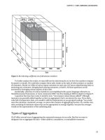
The decision tree is built as a series of splits, from left to right, as shown in Figure 11-12. The leftmost
node is All, which represents the entire campaign. The background color of each node is an indication of
that node’s population; the darker the color, the greater the population.

Please purchase PDF Split-Merge on www.verypdf.com to remove this watermark.
CHAPTER 11  DATA MINING
293
In your model, All is the darkest. To the right of All, the Clothing Buyer = 0 node is larger than
Clothing Buyer = 1. If you hover over Clothing Buyer = 0, an infotip will show the size of this node as
6,338. Doing this on the Clothing Buyer = 1 node will display 4,767.


Figure 11-12. Clothing Buyer = 0 node, with an infotip displayed
Each node in the bar under the node condition is a histogram that represents our buyers. The blue
portion of the bar is our True state, and the pink our False state. Click the All node and select Show
Legend. After the legend appears, dock it in the lower-right corner, as shown in Figure 11-13. Doing this
makes it easier to watch the values as you navigate the tree.

Please purchase PDF Split-Merge on www.verypdf.com to remove this watermark.
CHAPTER 11  DATA MINING
294

Figure 11-13. The Mining Legend, docked below the Solution Explorer
The Mining Legend has four columns of information about your model. The first column, Value,
shows 0, 1, and Missing. 0 is our false, or nonbuyer case, while 1 is our true, or buyer case. The Missing
value of 0 is good to see, as it indicates that our data is clean and fully populated. Our Cases column
displays the population of each case, and the Probability calculates this distribution as a percentage.
Finally, the Histogram column mimics the node’s histogram.
Reading the decision tree is done in a left-to-right manner, as shown in Figure 11-14. In our
Accessory Buyer model, the most significant factor that determines our accessory buyers is whether they
are also clothing buyers. This factor alone can enable the creation of a focused campaign. But in our
case, we see another valuable factor is at work here. The Number Children At Home node contains some
interesting values. The Number Children At Home >= 3 has a higher probability of purchase per its
Please purchase PDF Split-Merge on www.verypdf.com to remove this watermark.

CHAPTER 11  DATA MINING
295
histogram than the Number Children At Home < 3. On the other hand, the Number Children At Home <
3 is a darker node, meaning it has a greater population. Let’s take a closer look.
Click the Number Children At Home >= 3 node and review the Mining Legend. Our accessory buyers
equal 722, with a probability of 78.52 percent. Reviewing the Number Children At Home < 3 reveals 2,384
cases, with a probability of 61.95 percent. Based on these figures, your marketing group may decide to
target the group with fewer than three children at home first, because it has more buyers.


Figure 11-14. The decision tree is read in a left-to-right manner.
Using Drill-Through to View a Model’s Training Cases
Using drill-through, which you enabled when creating the AccessoryBuyers mining model, enables you
to see the underlying data that belongs to a particular node. Right-click the Number Children At Home <
3 node and select Drill Through, followed by Model Columns Only.
The Drill Through grid, shown in Figure 11-15, displays your training cases classified to Clothing
Buyer = 1 and Number Children At Home < 3. The model’s data points are displayed in alphabetical
order (I’ve hidden a few to narrow the view). Take note of the Number Children At Home column. It
Please purchase PDF Split-Merge on www.verypdf.com to remove this watermark.
CHAPTER 11  DATA MINING
296
contains values of 0, 1, and 2. This Number Children At Home bucket was created by the Decision Tree
algorithm during model processing.


Figure 11-15. The Drill Through grid, displaying the Number Children At Home < 3 node
■
Tip If you right-click on the grid contents and select Copy All, a copy of your cases will be placed into the copy
buffer, complete with column headings. This data can then be pasted into an Excel worksheet for further analysis.
Using the Dependency Network

You use the Dependency Network to view the input/predictable attribute dependencies in your model.
Clicking the Number Children At Home node will change the node display in the following ways:
Selected node: The background color will change to turquoise.
Predicts this node: If the selected node predicts this node, this node’s background color will change
to a slate-blue.

Next, click the Clothing Buyer node. Choosing Clothing Buyer will change the Dependency Network
view in the following ways:
Please purchase PDF Split-Merge on www.verypdf.com to remove this watermark.
CHAPTER 11  DATA MINING
297
Selected node: The background color will change to turquoise.
Predicts both ways: The selected node and this node predict each other. This node’s background
color is changed to purple.
Predicts the selected node: This node predicts the node you selected, and its background color is
changed to rust.

Finally, select the Accessory Buyer node, right-click, and select Copy Graph View. This copies your
Dependency Network, shown in Figure 11-16, to the Windows Clipboard.


Figure 11-16. The Dependency Network, with the Accessory Buyer node selected
The Mining Accuracy Chart View
The Mining Accuracy Chart tab, shown in Figure 11-17, is where you will validate your mining models.
For your Decision Tree model, you will be using the Input Selection and Lift Chart tabs. In the Input
Selection tab’s Predictable Column Name column, select Accessory Buyer. After this, select 1 for Predict
Value. From the Select Data Set to be Used for Accuracy Chart section, confirm that Use Mining Model
Test Cases is selected.

Please purchase PDF Split-Merge on www.verypdf.com to remove this watermark.

CHAPTER 11  DATA MINING
298

Figure 11-17. The Input Selection tab, displaying our prediction criteria
With the Input Selection tab completed, choose the Lift Chart tab. After a moment of processing, the
Data Mining Lift Chart for Mining Structure: AccessoryBuyersCampaign, and the Mining Legend that
you docked earlier will appear.
The lift chart, shown in Figure 11-18, will help you determine the value of your model. The lift chart
evaluates and compares your targets by using an ideal line and a random line. The percentage amount
difference between your lift line and your random line is referred to as lift in the marketing world. The
lift chart lines are defined as follows:
Random line: The random line is drawn as a straight diagonal line, from (0, 0) to (100, 100). For a
mining model to be considered a productive model, it should show some lift above this baseline.
Please purchase PDF Split-Merge on www.verypdf.com to remove this watermark.
CHAPTER 11  DATA MINING
299
Ideal line: Shown in green for this model this line reaches 100 percent Overall Population at 85
percent Target Population. The ideal line for the Accessory Buyers campaign suggests that a
perfectly constructed model would reach 100 percent of your targets by using only 85 percent of the
target population.
Lift line: This coral-colored line represents your model. The Accessory Buyers campaign follows the
ideal line for quite a ways, meaning that our model is performing quite well. Deciding to contact
more than 60 percent of the overall population will be a discussion point with marketing, because
this is where your model begins to trend back toward the random line.
Measured location line: This is the vertical gray line in the middle of the chart. This line can be
moved simply by clicking inside the chart. Moving this line will automatically update the Mining
Legend with the appropriate values.


Figure 11-18. The Accessory Buyers campaign lift chart

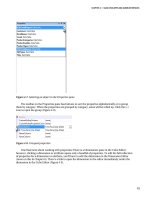
The Mining Model Prediction View
Now you are ready to create a prediction. Selecting the Mining Model Prediction tab displays the
Prediction Query Builder in Design view. Initially, there will be no selections in the Select Input Tables(s)
area, or in the Source/Field grid at the bottom of the designer.
To create your prediction query, complete the following steps:
Please purchase PDF Split-Merge on www.verypdf.com to remove this watermark.
CHAPTER 11  DATA MINING
300
1. Select a mining model: if AB_DecisionTree is not loaded in the Mining Model
box, click the Select Model button to navigate your data models. Expand the
AccessoryBuyersCampaign, and choose the AB_DecisionTree model.
2. Select your input table: in the Select Input Table(s) box, click the Select Case
Table button. In the Select Table dialog box, pick AccessoryCampaign from the
Data Source drop-down. After you have done this, choose the
ProspectiveBuyer table that marketing purchased, and click OK. Notice that
seven fields are automatically mapped between the mining model and the
ProspectiveBuyer table.
3. Map columns: in addition to the preceding columns that were mapped
automatically, we need to add our predict column. To do this, simply drag and
drop the Accessory Buyer column in your mining model onto the Unknown
column in the input table.
4. Design the query: In the Source/Field grid, you will select the specific data
points and data types to output for your prediction. Begin by choosing
Prediction Function from the Source drop-down list. In the Field drop-down
list, select PredictProbability. The last thing needed for our prediction function
is to drag and drop the Accessory Buyer column from the mining model to the
Criteria/Argument cell. Doing this will replace the cell’s text with
[AB_DecisionTree].[Accessory Buyer]. Next, you will add another row to the
grid. Choose AB_DecisionTree from the drop-down list in the row below
Prediction Function. In the Field column, ensure that Accessory Buyer is

chosen. You want to predict who your future buyers may be, so enter = 1 in the
Criteria/Argument column. Finally, you will want to identify your possible
customers. Do this by selecting ProspectiveBuyer in the next Source column,
and ProspectiveBuyerKey in the Field column.
5. Add other prospect information: Add additional customer information to the
grid by creating six new rows. For the first row, select ProspectiveBuyer as your
source, followed by FirstName as your field. Repeat the preceding steps five
more times, adding LastName, AddressLine1, City, StateProvinceCode, and
PostalCode.

When you have completed these steps, your Mining Model Prediction view should look like Figure
11-19.

Please purchase PDF Split-Merge on www.verypdf.com to remove this watermark.