Data Preparation for Data Mining- P8

H





M





L





Total

T




6





0





0





6

A




3





8





3





14

S




0





0





6





6

Total




9





8





9





26

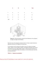
Figure 6.13 Bivariate histogram showing the joint distributions of the categories
for weight and height of the Canadiens.






Notice that some of the categories overlap each other. It is these overlaps that allow an
appropriate ordering for the categories to be discovered.




In this example, since the meaning of the labels is known, the ordering may appear
intuitive. However, since the labels are arbitrary, and applied meaningfully only for ease in
the example, they can be validly restated. Table 6.11 shows the same information as in
Table 6.10, but with different labels, and reordered. Is it now intuitively easy to see what
the ordering should be?

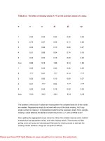
TABLE 6.11 Restated cross-tabulation.



Please purchase PDF Split-Merge on www.verypdf.com to remove this watermark.







A





B





C

Total








X




3





3





8

14





Y




0





6





0

6





Z




6





0





0

6





Total




9





9





8





26

Table 6.11 contains exactly the same information as Table 6.10, but has made intuitive
ordering difficult or impossible. It is possible to use this information to reconstruct an
appropriate ordering, albeit not intuitively. For ease of understanding the previous labeling
system is used, although the actual labels used, so long as consistently applied, are not
important to recovering an ordering.




Restating the cross-tabulation of Table 6.10 in a different form shows how this recovery
begins. Table 6.12 lists the number of players in each of the possible categories.




TABLE 6.12 Category/count tabulation.

Weight




Height





Count








H




T

6





H




A





3





H

S





0





M




T





0





M

A





8





M




S





0

Please purchase PDF Split-Merge on www.verypdf.com to remove this watermark.


L




T





0





L




A

3





L




S





6








The information in Table 6.12 represents a sort of jigsaw puzzle. Although in this example
the categories in all of the tables are shown appropriately ordered to clarify explanation,

the real situation is that the ordering is unknown and that needs to be discovered. What is
known are the various frequencies for each of the category couplings, which are pairings
here as there are only two variables. From these, the shape of the jigsaw pieces can be
discovered.




Figure 6.14(a) shows the pieces that correspond to Weight = “H.” Altogether there are
nine players with weight “H.” Six of them have height “T,” three of them have height “A,”
and none of them have height “S.” Of the three possible pieces corresponding to H/T,
H/A, and H/S, only the first two have any players in them. The figure shows the two
pieces. Inside each box is a symbol indicating the label and how many players are
accounted for. If the symbols are in brackets, it indicates that only part of the total number
of players in the class are accounted for. Thus in the left-hand box, the top (6H) refers to
six of the players with label “H,” and there remain other players with label “H” not
accounted for. The lower 6T refers to all six players with height label “T.” The dotted lines
at each end of the incomplete classes indicate that they need to be joined to other pieces
containing members of the same class, that is, possessing the same label. The dotted
lines are at each end because they could be joined together at either end. Similar pieces
can be constructed for all of the label classes. These two example pieces can be joined
together to form the piece shown in Figure 6.14(b).







Please purchase PDF Split-Merge on www.verypdf.com to remove this watermark.

Figure 6.14 Shapes for all players with weight = “H” (a), two possible assembled
shapes for the 9H/6T/3A categories (b), shapes created for each of the category
combinations (c), fitting the pieces together recovers an appropriate ordering (d),
and showing a straight-forward way of finding a numeration of each variable’s
three segments (e).






Figure 6.14(b) shows the shape of the piece for all players with Weight = “H.” This is built
from the two pieces in Figure 6.14(a). There are nine players with weight “H.” Of these, six
have height “T” and three have height “A.” The appropriate jigsaw piece can be
assembled in two ways; the overlapping “T” and “A” can be moved. Since the nine “H”
(heavy) players cover all of the “T” (tall) players, the “H” and “T” parts are shown drawn
solidly. The three “A” are left as part of some other pairing, and shown dotted. Similar
shapes can be generated for the other category pairings. Figure 6.14(c) shows those.




For convenience, Figure 6.14(c) shows the pieces in position to fit together. In fact, the
top and bottom sections can slide over each other to appropriate positions. Fitting them
together so that the matching pieces adjoin can only be completed in two ways. Both are
identical except that in one “H” and “T” are on the left, with “S” and “L” on the right. The
other configuration is a mirror image.

Fitting the pieces together reveals the appropriate order for the values to be placed in
relation to each other. This is shown in Figure 6.14(d). Which end corresponds to “0” and
which to “1” on a normalized scale is not possible to determine. Since in the example
there are only three values in each variable, numerating them is straightforward. The
values are assigned in the normalized range of 0–1, and values are assigned as shown in
Figure 6.14(e).




Having made an arbitrary decision to assign the value 0 to “H” and “T,” the actual
numerical relationship in this example is now inverted. This means that larger values of
weight and height are estimated as lower normalized values. The relationship remains
intact but the numbers go in the “wrong” direction. Does this matter? Not really. For
modeling purposes it is finding and keeping appropriate relationships that is paramount. If
it ever becomes possible to anchor the estimated values to the real world, the accuracy of
the predictions of real-world values is unaffected by the direction of increase in the
estimates. If the real-world values remain unknown, then, when numeric predictions are
made by the final model, they will be converted back into their appropriate alpha value,
which is internally consistent within the model. The alpha value predictions will be
unaffected by the internal numerical representation used by the model.




Although very simplified, how well does this numeration of the alpha values work? For
convenience Table 6.13 shows the normalized weights and normalized heights with the

estimated valves uninverted. This makes comparison easier.


Please purchase PDF Split-Merge on www.verypdf.com to remove this watermark.


TABLE 6.13 Comparison of recovered values with normalized values.







Normalized
height




Estimated
height





Normalized
weight

Estimated
weight








1




1





1

1





0.759036




1





0.876923





1

0.698795




1





0.769231





1





0.698795




1

0.753846





1





0.698795




1





0.692308

1





0.698795




1





0.692308





1

0.60241




0.5





0.753846





1





0.60241

0.5





0.523077





0.5





0.60241




0.5





0.384615

0.5





0.493976




0.5





0.846154





1

0.493976




0.5





0.692308





1





0.493976

0.5





0.615385





0.5





0.493976




0.5

0.538462





0.5





0.493976




0.5





0.538462

0.5





0.493976




0.5





0.492308





0.5





0.493976

0.5





0.446154





0.5





0.493976




0.5

0.323077





0









Please purchase PDF Split-Merge on www.verypdf.com to remove this watermark.

0.493976



0.5



0.323077

0




0.39759




0.5





0.369231





0.5

0.39759




0.5





0.184615





0





0.301205




0

0.276923





0





0.301205




0





0

0





0.192771




0





0.246154





0

0.192771




0





0.230769





0





0.192771

0





0.184615





0





0




0

0.107692





0








6.3.2 More Values, More Variables, and Meaning of the
Numeration




The Montreal Canadiens example is very highly simplified. It has a very small number of
instance values and only three alpha values in each variable. In any practically modelable
data set, there are always far more instances of data available and usually far more
variables and alpha labels to be considered. The numeration process continues using
exactly the same principles as just described. With more data and more variables, the
increased interaction between the variables allows finer discrimination of values to be
made.

What has using this method achieved? Only discovering an appropriate order in which to
place the alpha values. While the ordering is very important, the appropriate distance
between the values has not yet been discovered. In other words, we can, from the
example, determine the appropriate order for the labels of height and weight. We cannot
yet determine if the difference between, say, “H” and “M” is greater or less than the
difference between “M” and “L.” This is true in spite of the fact that “H” is assigned a value
of 1, “M” of 0.5, and “L” of 0. At this juncture, no more can be inferred from the assignment
H = 1, M = 0.5, L = 0 than could be inferred from H = 1, M = 0.99, L = 0, or H = 1, M = 0.01,
L = 0.




Something can be inferred about the values between variables. Namely, when normalized
values are being used, both “H” and “T” should have about the same value, and “M” and
“A” should have about the same value, as should “L” and “S.” This does not suggest that

Please purchase PDF Split-Merge on www.verypdf.com to remove this watermark.
they share similar values in the real world, only that a consistent internal representation
requires maintenance of the pattern of the relationship between them.



Even though the alpha labels are numerically ordered, it is only the ordering that has
significance, not the value itself. It is sometimes possible to recover information about the
appropriate separation of values in entirely alpha data sets. However, this is not always
the case, as it is entirely possible that there is no meaningful separation between values.
That is the inherent nature of alpha values. Steps toward recovering appropriate

separation of values in entirely alpha data sets, if indeed such meaningful separation
exists, are discussed in the next chapter dealing with normalizing and redistributing
variables.




6.3.3 Dealing with Low-Frequency Alpha Labels and Other
Problems




The joint frequency method of finding appropriate numerical labels for alpha values can
only succeed when there is a sufficient and rich overlap of joint distributions. This is not
always the case for all variables in all data sets. In any real-world data set, there is always
enough richness of interaction among some of the variables that it is possible to numerate
them using the joint frequency table approach. However, it is by no means always the
case that the joint frequency distribution table is well enough populated to allow this
method to work for all variables. In a very large data set, some of the cells, similar to those
illustrated in Figure 6.13, are simply empty. How then to find a suitable numerical
representation for those variables?




The answer lies in the fact that it is always possible to numerate some of the variables using
this method. When such variables have been numerated, then they can be put into a
numerical form of representation. With such a representation available in the data set, it
becomes possible to numerate the remaining variables using the method discussed in the

previous section dealing with state space. The alpha variables amenable to numeration
using the joint frequency table approach are numerated. Then, constructing the manifold in
state space using the numerated variables, values for the remaining variable instance values
can be found.


6.4 Dimensionality




The preceding two parts of this chapter discussed finding an appropriate numerical
representation for an alpha label value. In most cases, the discovered numeric
representation, as so far discussed, is as a location on a manifold in state or phase space.
This representation of the value has to be described as a position in phase space, which
takes as many numbers as there are dimensions. In a 200-dimensional space, it would
take a string of 200 numbers to indicate the value “gender = F,” and another similar string,
with different values, to indicate “gender = M.” While this is a valid representation of the
alpha values, it is hopelessly impractical and totally intractable to model. Adding 200

Please purchase PDF Split-Merge on www.verypdf.com to remove this watermark.
additional dimensions to the model simply to represent gender is impossible to deal with
practically. The number of dimensions for alpha representation has to be reduced, and
the method used is based on the principles of multidimensional scaling.



This explanation will use a metaphor different from that of a manifold for the points in
phase space. Instead of using density to conjure up the image of a surface, each point will
be regarded as being at the “corner” of a shape. Each line that can be drawn from point to

point is regarded as an “edge” of a figure existing in space. An example is a triangle. The
position of three points in space can be joined with lines, and the three points define the
shape, size, and properties of the triangle.




6.4.1 Multidimensional Scaling




MDS is used specifically to “project” high-dimensionality objects into a lower-dimensional
space, losing as little information as possible in the process. The key idea is that there is
some inherent dimensionality of a representation. While the representation is made in
more dimensions than is needed, not much information is lost. Forcing the representation
into less dimensions than are “natural” for the representation does cause significant loss,
producing “stress.” MDS aims at minimizing this stress, while also minimizing the number
of dimensions the representation needs. As an example of how this is done, we will
attempt to represent a triangle in one dimension—and see what happens.




6.4.2 Squashing a Triangle




A triangle is inherently a 2D object. It can be defined by three points in a state or phase

space. All of the triangular points lie in a plane, which is a 2D surface. When represented
in three dimensions, such as when printed on the page of this book, the triangle has some
minute thickness. However, for practical purposes we ignore the thickness that is actually
present and pretend that the triangle is really 2D. That is to say, mentally we can project
the 3D representation of a triangle into two dimensions with very little loss of information.
We do lose information about the actual triangle, say the thickness of the ink, since there
is no thickness in two dimensions. Also lost is information about the actual flatness, or
roughness, of the surface of the paper.




Since paper cannot be exactly flat in the real world, the printed lines of the triangle are
minutely longer than they would be if the paper were exactly flat. To span the miniature
hills and valleys on the paper’s surface, the line deviates ever so minutely from the
shortest path between the two points. This may add, say, one-thousandth of one percent
to the entire length of the line. This one-thousandth of one percent change in length of the
line when the triangle is projected into 2D space is a measure of the stress, or loss of
information, that occurs in projecting a triangle from three to two dimensions. But what
happens if we try to project a triangle into one dimension? Can it even be done?




Figure 6.15 shows, in part, two right-angled triangles that are identical except for their

Please purchase PDF Split-Merge on www.verypdf.com to remove this watermark.
orientation. The key feature of the triangles is the spacing between the points defining the
vertices, or “corners.” This information, or as much of it as possible, needs to be
preserved if anything meaningful is to be retained about the triangle.

Figure 6.15 The triangle on the left undergoes more change than the triangle on
the right when projected into one dimension. Stress, as measured by the change
in perimeter, is 33.3% for the triangle on the left, but only 16.7% for the triangle on
the right.






To project a triangle from three to two dimensions, imagine that the 3D triangle is held up
to an infinitely distant light that casts a 2D shadow of the triangle. This approach is taken
with the triangles in Figure 6.15 when projecting them into one dimension.




Looking at the orientation 1 triangle on the left, the three points a, b, and c cast their
shadows on the 1D line below. Each point is projected directly to the point beneath. When
this is done, point a is alone on the left, and points b and c are directly on top of each
other. What of the original relationship is preserved here?

The original distance between points a and c was 5. The projected distance between the
same points, when on the line, becomes 4. This 5 to 4 change in length means that it is
reduced to 4/5 of its original length, or by 1/5, which equals 20%. This 20% distortion in
the distance between points a and c represents the stress on this distance that has
occurred as a result of the projection.




Each of the distances undergoes some distortion. The largest change is c to b in going
from length 3 to length 0. This amount of change, 3 out of 3 units, represents a 100%
distortion. On the other hand, length a to b experiences a 0% distortion—no difference in
length before and after projection.




The original “perimeter,” the total distance around the “outside” of the figure was


Please purchase PDF Split-Merge on www.verypdf.com to remove this watermark.


a to b = 4

b to c = 3




c to a = 5




for a total of 12. The perimeter when projected into the 1D line is




a to b = 4




b to c = 0




c to a = 4

for a total of 8.




So the change in perimeter length for this projection is 4, which is the difference of the
before-projection total of 12 and the after-projection total of 8.




The overall stress here, then, is determined by the total amount of change in perimeter
length that happened due to the projection:




change in length = 4




original length = 12




change = 4/12

or 33%. Altogether, then, projecting the triangle with orientation 1 onto a 1D line induced a
33% stress. Is this amount of stress unavoidable?




The triangle in orientation 2 is identical in size and properties to the triangle in orientation
1, except that it was rotated before making the projection. Due to the change in
orientation, points b and c are no longer on top of each other when projected onto the line.
In fact, the triangle in this orientation retains much more of the relationship of the
distances between the points a, b, and c. The a to b distance retains the correct
relationship to the b to c distance, although both distances lose their relationship to the a
to c distance. Nonetheless, the total amount of distortion, or stress, introduced in the
orientation 2 projection is much less than that produced in the orientation 1 projection.
The measurements in Figure 6.15 for orientation 2 show, by reasoning similar to that
above, that this projection produces a stress of 16.7%. In some sense, making the
projection in orientation 2 preserves more of the information about the triangle than using
orientation 1.


Please purchase PDF Split-Merge on www.verypdf.com to remove this watermark.


The important point about this example is that changing the orientation, that is, rotating
the object in space, changes the amount of stress that a particular projection introduces.
For most such objects this remains true. Finding an optimal orientation to reduce the
stress of projection is important.

6.4.3 Projecting Alpha Values




How does this example relate to dimensionality reduction and appropriate representation
for alpha labels?




When using state space to determine values for alpha labels, the method essentially finds
appropriate locations to place the labels on a high-dimensionality manifold. Each label
value has a more or less unique position on the manifold. Between each of these label
locations is some measurable distance in state space. Using the label positions as points
on the manifold, distances between each of the points can easily be discovered using the
high-dimensional Pythagorean theorem extension. These points, with their distances from
each other, can be plucked off the state space manifold, and the shape represented in a
phase space of the same dimensionality. From here, the principle is to rotate the shape in
its high-dimensional form, projecting it into a lower-dimensionality space until the
minimum stress level for the projection is discovered. When the minimum stress for some
particular lower dimensionality is discovered, if the stress level is still acceptable, a yet
lower dimensionality is tried, until finally, for some particular lower dimensionality, the
stress becomes unacceptably high. The lowest-dimensionality representation that has an
acceptable level of stress is the one deemed appropriate to represent the alpha variable.
(What might constitute an acceptable level of stress is discussed shortly.)

6.4.4 Scree Plots




The idea that stress changes with projection into lower numbers of dimensions can
actually be graphed. If a particular shape is projected into several spaces of different
dimensionality, then the amount of stress present in each space, plotted against the
number of dimensions used for the projection, forms what is known as a scree plot. Figure
6.16 shows just such a plot.







Please purchase PDF Split-Merge on www.verypdf.com to remove this watermark.


Figure 6.16 Ideal scree plot.

Starting with 30 dimensions in Figure 6.16, a high-dimensional figure is projected into
progressively fewer dimensions. Not much change occurs in the level of stress
occasioned by the change in dimensionality until the step from five to four dimensions. At
this step there is a marked change in the level of stress, which increases dramatically with
every reduction from there.




The step from five to four dimensions is called a knee. In dimensionalities higher than this
knee, the object can be accommodated with little distortion (stress). Clearly, four
dimensions are not sufficient to adequately represent the shape. It appears, from this
scree plot, that five is the optimum dimensionality to use. In some sense, a
five-dimensional representation is the best combination of low dimensionality with low
stress.




When it works satisfactorily, finding a knee in a scree plot does provide a good way of
optimizing the dimensionality of a representation. In practice, few scree plots look like
Figure 6.16. Most look more like the ones shown in Figure 6.17. In practice, finding
satisfactory knees in either of these plots is problematic. When satisfactory knees cannot
be found, a workable way to select dimensionality is to select some acceptable level of
stress and use that as a cutoff criterion.

Figure 6.17 Two more realistic scree plots.


6.6 Summary




This chapter has covered a lot of ground in discussing the need for, and method of,
finding justifiable numeric representations of alpha-valued variables. The concepts of
methods for performing this numeration in mixed alpha-numeric and in entirely alpha data

Please purchase PDF Split-Merge on www.verypdf.com to remove this watermark.